|
A Guide to Implementing the Theory of
Constraints (TOC) |
|||||
Evaluating Change When we set out to implement
change we must remember that there are 3 possible outcomes. These outcomes are; (1) A
change which is a significant improvement. (2) A
change which is neither a significant improvement nor a significant decline. (3) A
change which is a significant decline. Naturally enough, it is
the first option that we are really seeking.
We want to make a difference, and we want that difference to be
manifestly positive. In order to do
so, we must make decisions prior to carrying out the desired actions, and to
be certain in the knowledge that those decisions will deliver the necessary
results that we seek. How we evaluate the
improvement will depend upon the goal of the system. If the goal is a monetary one, then the
evaluation is relatively straightforward.
And that is what we will concentrate on here. In not-for-profit, or more correctly,
for-cause situations how we evaluate an improvement is a little more
involved; however, if you look at the argument for healthcare (supply chain
section) then you will find some good indications of how this can be
achieved. We are evaluating changes
within the context of the whole system – or the system as a whole. We are not interested in local improvements
that do not have system-wide impact.
How, then, would we judge an impact in such a circumstance? We need a context. We already have one, let’s revisit it. On the measurements page
we derived our rules of engagement.
These tell us how to define the entity that we want to improve. We define the boundaries, the goal, the
necessary conditions, and the fundamental measurements. Without these, we do not have a context
within which to evaluate change.
Moreover, this forces us to determine what it is that constrains us
from moving towards our goal; we have to define the role of the constraints. The constraints are
central to our ability to move forward.
In order to define the role of the constraints we need to invoke our
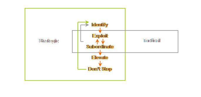
plan of attack, the one we developed on the process of change page. Of course, our plan of attack is Goldratt’s
focusing process. The second step of
this plan, where we decide how to exploit the constraints, is the step that
provides commonality between these two schemes. We have previously
summarized the relationship between the rules of engagement and the plan of
attack as follows;
In order for a change to be
an improvement it must either have a direct positive effect upon the current
exploitation or elevation of the system’s constraints, or an indirect effect
via improved subordination which in-turn ought to improve the exploitation or
elevation, either now or in the future.
To quantify these effects
we must return to our fundamental measurements. In the first page, the
page on measurements, we briefly introduced the concepts of; throughput, inventory/investment,
and operating expense; a triumvirate set
of measures for quantifying effects in Theory of Constraints. Throughput as you may
remember was described as; Throughput
= Sales - Totally Variable Costs From this we came to
define our net profit as; Net Profit
= Throughput - Operating Expense And return-on-investment
is;
The reason that we can do
so much with so little is because of the fundamental relationships that exist
between each measure. They are systemic. Let’s try to reinforce
the fundamental and systemic nature of these measures by way of analogy. By this means we will be in a far stronger
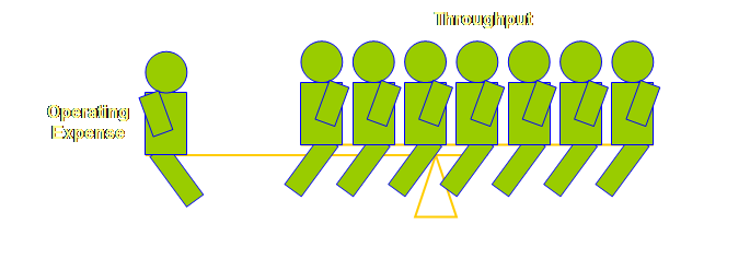
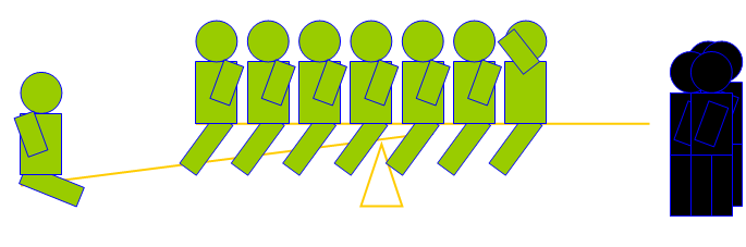
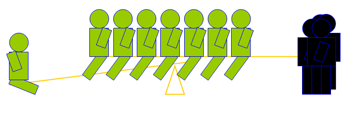
position to understand change and how to evaluate it. The analogy is a see-saw. A see-saw!
How does the evaluation of change relate to a see-saw? Well, let’s have a look. Let’s draw a simple see-saw as a start.
The two equal masses – “people” are located
equidistant from the mid-point of the plank, so let’s label that.
Let’s see.
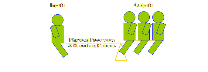
Can we use this simple analogy of a see-saw for
evaluating internal management decisions, change in other words? In terms of physical
aspects it is apparent that we seek to leverage inputs of some
kind via a process of some sort in order to produce outputs. In fact, the process does not exist in
isolation but rather it exists in conjunction with a set of operating
assumptions; the things that we call policies. How then would this look using our
model? Let’s see.
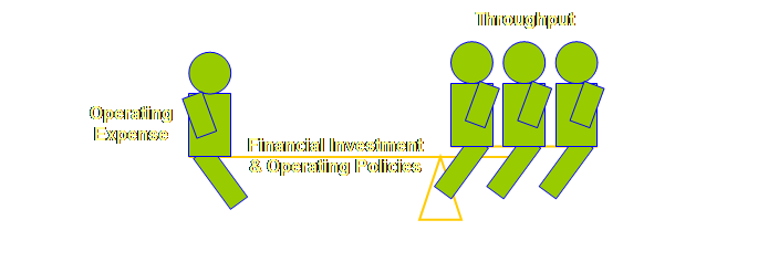
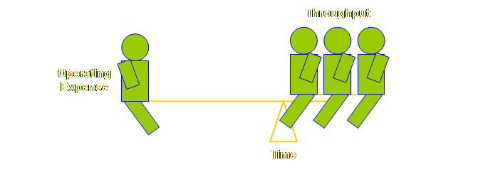
How then would our model look in terms of financial
aspects? In the terms of financial aspects it is apparent that we seek to leverage
expenditure via investment to produce income.
Once again the investment does not exist in isolation but rather it
exists in conjunction with a set of working assumptions; policies once
again. Let’s see how this looks.
We need to ask then; will this simple analogy, a
see-saw, also work as a description for evaluating change in Theory of
Constraints? Well, I think so, so
let’s try.
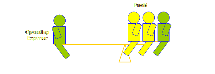
It seems then, that our analogy will hold for our fundamental
measures. Great. Any change in throughput, or operating expense may
change the balance of our system. Do
you agree? Our analogy shows the
interrelationships between these various aspects. Do you want to push the analogy a little bit
further? What is our profit then? Let’s have a look.
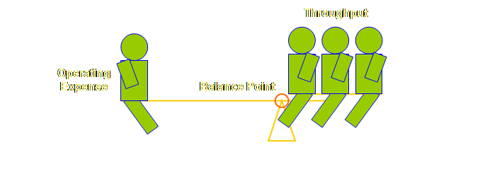
What about the balance point then?
We know the location of the balance point, but this
begs a question. What is the fulcrum
that we leverage across? Let’s have a look.
I know that all too often we loosely talk about
leveraging the constraint – we have used that language throughout these
webpages and it is probably ingrained.
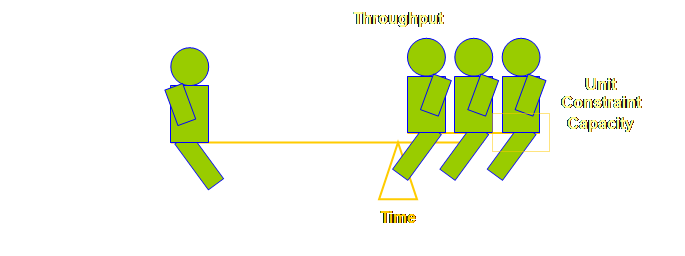
But in reality we are leveraging our entire system
over the fulcrum – time – and the only
way that we can do that, either literally or metaphorically, is via the
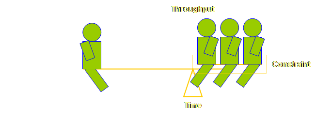
constraint. So we leverage the
system via the constraint for a given unit of time. So, yet another question; what exactly is the
constraint in our analogy then?
Now that we have identified
the constraint, how can we get more of this limiting factor? How in our metaphor can we get more people
sitting balanced on the right-hand side?
How can we improve the Throughput?
How can we improve the profit?
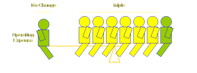
There are two answers to these questions, and they are that we can
increase the productivity, and/or we can increase the production. We need to tease these two strands apart in
order to better understand each of them.
Let’s do that. Making a distinction between productivity and
production is important in understanding how to most effectively drive
improvement, and such a distinction is also useful in developing our
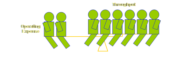
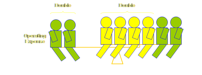
understanding of the dynamics of exploitation, subordination, and elevation. Production is the simpler, and certainly
more familiar of the two concepts, so let’s start with that. Essentially any increase in production is a pro rata
increase in both inputs (operating expense), and outputs (Throughput). Let’s investigate this with our see-saw
analogy. Let’s start again with our original model with a
balance point located 3/4 of the way along the plank.
Increasing production, seductive as it is – after
all this is what almost everybody else does – is nowhere near as sexy as
improving productivity per se.
Moreover, if we were to go around doing what everyone else does then
there is hardly any strategic advantage to be had at all. So let’s investigate the impact of
improving productivity; many people talk about increasing productivity but
few actually manage to do it. Doing it
is not at all difficult if we have focus. Rather than settling for a pro rata increase in both
operating expense and throughput, which means constant productivity – only
more of it, we actively seek to decouple throughput from operating expense,
which in-turn means increased productivity.
Throughput should increase and ideally operating expense should remain
static or even decrease; something other than additional operating expense
drives the additional throughput. It
is the leveraging of the entire system via the constraint’s throughput
relative to the fulcrum, time, that drives the additional throughput. Let’s show this by example. Let’s start again with our original model with a 3:1
ratio.
An increase in productivity will in-turn
substantially increase profit. Let’s
have a look at that.
We obtain better leverage by better exploitation of the constraint (the secondary plank
becomes longer) and by better subordination
of the non-constraints. Often the
simplest way to obtain an increase in leverage is to remove or modify some
current policy. Organizations abound
with policy; that is, after all, one way in which to standardize matters, and
without standardization there can be no base from which to improve. But what if the standardization causes us
to stagnate instead of improve? Policy
also allows us to react quickly without reinventing the wheel each time. But what if we no longer need a particular
reaction and yet we still have the policy?
Removal of outdated or inappropriate policy unblocks access to current
capacity and increases productivity. Now, if we are still bored with our newfound
increase in productivity, then we can still increase our production after we have increased our productivity – given that our
capacity allows for it. It pays in
more ways than one to increase relative productivity first, and then absolute
production second, rather than the other way around. Always aim for capability before capacity. That is why the 5 focusing steps; our plan of attack
goes; identify, exploit/subordinate, elevate
– in that order. Most firms go;
identify, elevate – every time. In
fact that is unfair, most firms miss the identification stage and have a
scatter gun approach of; elevate, elevate, elevate. Hardly a wise use of cash, and a total
absence of any systematic decision analysis. In reality, often both productivity and production
are inexorably mixed together, but we need to understand the dynamics of each
component if we are to better understand how to correctly influence the whole
– even if later on we can’t so neatly break the whole back into constituent
parts as we have here. It is apparent from the logic of this discussion
that as the lever moves with respect to the fulcrum; the productivity, throughput,
and hence profit, should trend towards infinity. But we are getting ahead of ourselves. None of us are making infinite profits yet
(or if we are, then we certainly haven’t told Inland Revenue about it). So, this begs a question. Why aren’t we making infinite profits yet? Well, a valid reason might be a finite
capacity or capability of the current constraint; we are unable to move the
balance point any closer to the end of the lever. We can neither exploit the constraint nor
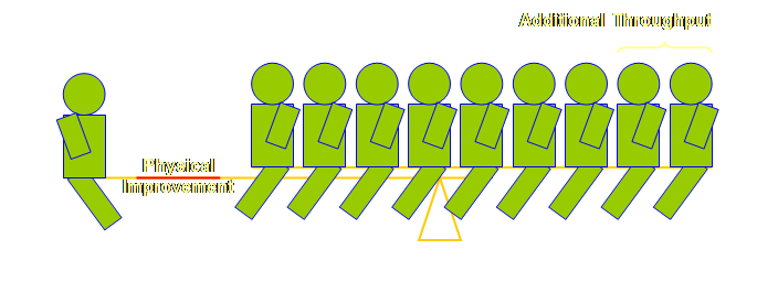
subordinate the system any further, even though the demand is there? What shall we do? Well, why don’t we make the lever even longer? Let’s have a look at a new aspect;
investment. In our analogy additional investment means that our
lever becomes a little longer. The
effect of the investment in this instance is to both exploit
& elevate the existing constraint or to better subordinate the
non-constraints which in-turn exploits the constraint. Let’s work from our current state where we
have 7/8’s of the lever on one side and 1/8 on the other. Here is our starting point.
The effect of the investment is to increase the
physical leveragability of the system even though the absolute position of
the balance point remains static.
Effectively we have increased the productivity of the system by
capital investment. This is
interesting (to me). Here we have both
elevation (cash from outside the
system was brought inside – even though it is not an increase in operating
expense) and exploitation (the absolute
position of the balance point did not change, but the position relative to
the whole plank did change). Alright, maybe that is pushing our metaphor
about as far as it should go at the moment. Let’s now return to the formulae that express the
reality of these simple diagrams to further evaluate the situation. We introduced 3 equations in the section on
fundamental measurements, let’s repeat two of them here, one for throughput
and one for profit (or operating surplus); Throughput
= Sales - Totally Variable Costs and Net Profit
= Throughput - Operating Expense Of course we can combine these into one statement Net Profit
= Sales - Totally Variable Costs - Operating
Expense However, let’s confine ourselves to the simpler
version Net Profit
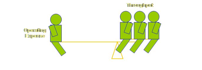
= Throughput - Operating Expense And let’s compare this directly with the simplest of
our see-saw analogies. Here is the
analogy.
Net Profit = 3 Units of
Throughput - 1 Unit of Operating Expense
= 2 Units Just as we drew it,
We can see that the fulcrum is represented in the
diagrams and we can see that its positioning under the balance point is
critical, and we know that it represents time, yet it seems to disappear from
our equations. Let’s clarify this
issue. The fulcrum is time – the one thing we don’t seem to
be able to generate any additional quantity of, and time is present in our
equations, but we seem to have been a little lax in making it explicit. Really our equations should read as
follows. Throughput should be;
And one again, if we combine these equations we get;
We are more interested in evaluating change before
we make the change. We want to know
the outcome of a potential decision before we take action to implement it as
an actual decision. And for this we
need some critical information. We need to be able to determine the Throughput
through a unit of constraint capacity in relation to time.
This is the major
decision analysis that we make. We
need to examine this in detail. Let’s return to our original case for a moment.
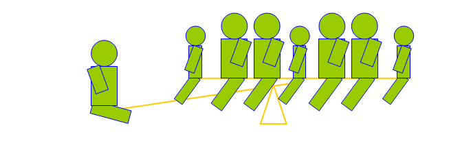
Upon the improved leverage of the example above we
found the following;
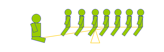
But equally, we might also have found this;
If we substituted children for all of the adults we
could even have found this;
How can we know ahead of time what the outcome of
these types of substitutions will be?
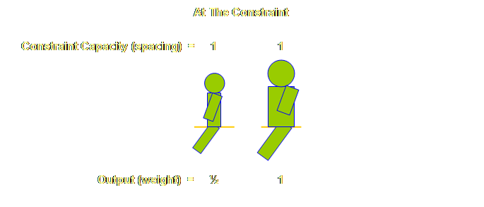
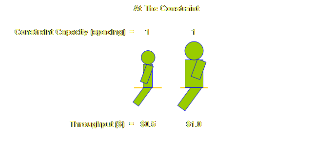
Graphically it seem obvious, we need to know the output value, the
weight, for each type of output in this system relative
to the unit constraint capacity. Let’s show this.
It is a simple step to move our analogy from output
to throughput so that we can evaluate the financial
aspects. Let’s have a look.
We have produced a normalized throughput per unit of
output as viewed from the perspective of the constraint. But, we have
nearly lost sight of our fulcrum (again).
What has happened to our measure of time? Mention was made of the short-hand expression “T/cu”
or Throughput per constraint unit earlier.
This short-hand is partially responsible for the apparent lack of
time. It is there, however. The full expression should be “throughput
per constraint unit per unit time,” or T/cu/t. In our simple analogy our constraint unit is
seating, and thus we would evaluate Throughput as Throughput $ per seat per
ride. “Seat” is the constraint unit,
“ride” is the expression for time. Let’s look at a few other general cases. What about a sunshine factory? And by that I mean an outdoor agricultural
or horticultural enterprise. The
constraint unit here is available productive area, and the decision analysis
becomes Throughput $ per acre or hectare per season or per year (T$/hectare/year). What about an indoor retail operation? Something that doesn’t make anything; just
buys and sells. The constraint unit
here is again productive area, if might be square meters or square feet of
floor space, or square meters or square feet of shelf space if there is a
vertical component as well, and the decision analysis becomes Throughput $
per square meter per week or per month depending on the rate of turnover (T$/m2/week).
Supermarkets tend to use linear meters of “facing” assuming that we
buy in proportion to what we see. If
the facing all has the same volume stacked behind it, then there would seem
to be little difference in the various units. Larger items in a sales system where a sale is
concluded after a sales process, then the constraint should be the number of
contact sales hours that the sales people have. The decision analysis becomes Throughput $
per sales person per hour or day (T$/sales person/hour). In manufacturing the constraint is most usually a
machine or group of machines and this is the constraint unit, the unit of
time is most commonly minutes because manufacturing steps are more commonly
completed within minutes or hours rather than days. The throughput decision analysis becomes
Throughput $ per machine per minute (T$/machine/minute). Some examples that I know of are
people-paced rather than machine-paced and the throughput decision analysis
becomes Throughput $ per man per hour (T$/man/hour). What then of projects? The constraint is the number of resources
working on the critical chain. The
Throughput decision analysis becomes Throughput $ per critical chain person
per project week or month (T$/critical chain
person/month). Remember these are decision analyses; the analysis
of various choices before we
embark on a decision. Once we have
made a commitment to the customer we can’t internally re-prioritize according
these values. With this new information under our belt, now, at
least, we can predict the Throughput for the following case before we
actually do it.
What about the other case?
Graphically this is just plain obvious, we can see,
and we know from our own direct experience with see-saws. But trust me, in most organizational
systems this is anything but clear, and one good reason for this is that
almost no one in most organizations has ever considered this before. “We have to evaluate the impact, not of a product,
but of a decision. This evaluation
must be done through the impact on the system’s constraints. That’s why identifying the constraints is
always the first step (1).” We have to know
where the constraint, is; and we have to know
the Throughput value of the output with respect to that constraint. So, anyone can
work out the Throughput retrospectively for any period. No one can
evaluate the Throughput proactively for the current or future periods without
explicit knowledge of the Throughput value generated with respect to the
constraint. In some instances this
might be quite obvious; most often, however, it is not. And when it is done there are most often
some surprises in the relative ranking of the outputs. This brings us to a very important point. We all know from our own personal experiences with
see-saws, that if we change just one important thing then the whole balance
may change. If we move the plank a
little, or if someone gets on, or if someone gets off, or even it someone
changes ends, then, so too, does the balance.
And so too, with our system under investigation. We didn’t know previously that once we elevated this
system that children might get on, or that adults might get off. But every time we prepare to change the
constraint that is exactly what we must evaluate for. We must evaluate for the new mix that could
arise. If we think that we will
elevate a constraint to the extent that we will break it (and thus a new
constraint presents itself) then the unit throughput values, and thus the
individual ranking, may also change and therefore maybe also our tactics for exploitation
will change as well. We must predict the outcome ahead of implementing
the decision. “You see, in the ‘cost
world’ almost everything is important, thus changing one or two things
doesn’t change the total picture much.
But this is not the case in the ‘throughput world.’ Here, very few things are really
important. Change one important thing
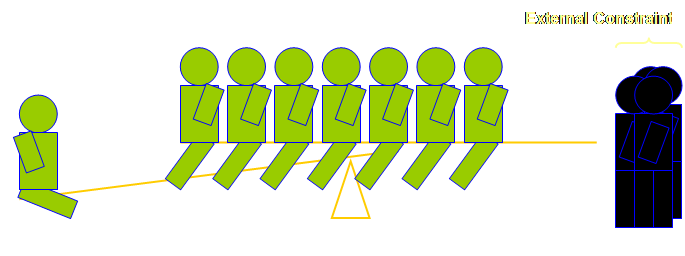
and you must re-evaluate the entire situation (2).” In internally constrained systems we can not satisfy
market demand. We can show this with
our analogy? Of course we can. The beam is full, we could get other people
on, if only they would fit.
We have, loosely speaking, begun to evaluate
decisions about the composition of the physical output – the so-called
production mix. Now, there is almost
nothing, either positive or negative, that a good production manager can not
ascribe, in one way or another, to the changes in the production mix. The production manager can do this without
fear of contradiction because, in fact, almost no one else understands the
true impact of the production mix – often not even the production manager! But we do understand – only too well. We do, because we know how to strip out all of the
raw material costs or 1:1 variable costs in the production mix leaving
us with the bare essentials – we could call this the throughput mix
(3, 4). Moreover, we know that we must
evaluate the throughput mix in relation to one thing and one thing only, the
amount of resource consumed to produce the throughput mix on the constraint. Let’s therefore look at this in a little more
detail. We need to better delineate
some aspects that are particularly important in internally constrained
environments. Maybe we should describe
these as generic tactics. We need to do this in order to later
appreciate some of the subtle changes that occur in the tactics once a system
becomes externally constrained. It becomes part of the exploitation strategy of
internally constrained systems to maximize the throughput mix by including,
as much as possible, products that generate high throughput per unit time on
the constraint; these are the adults of our analogy. In shorthand we might describe these as
high “T/cu” products, where “T” means throughput and “cu” means constraint
unit. We saw this aspect demonstrated
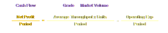
so well in the P & Q analysis. However, I want to introduce the word “grade” to
describe this aspect of throughput mix.
We want to substitute, wherever possible, higher grade unit throughput
for lower grade unit throughput. We
want to produce “stars” not “dogs” if the market will allow us – and it
should. The overall grade is a
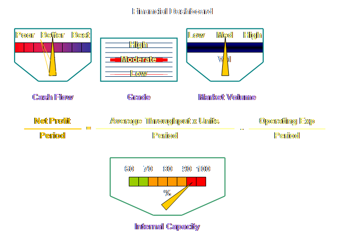
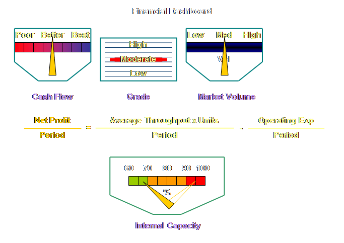
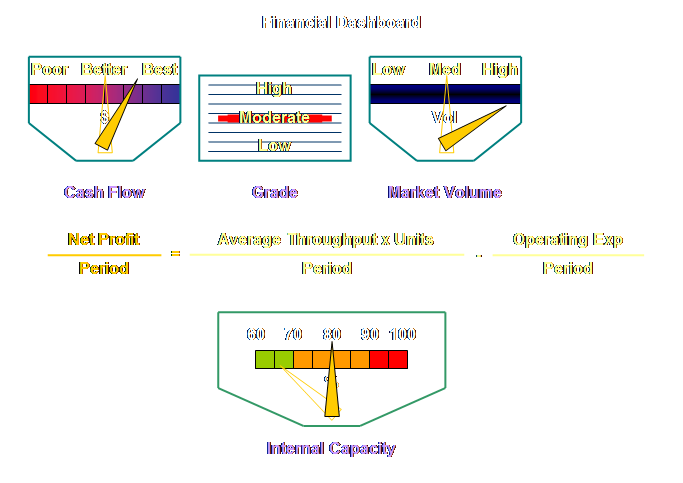
reflection of the average throughput per unit. Moreover, let’s call the current market capacity
“market volume” and the profit “cash flow.”
Let’s have a look at the relationships.
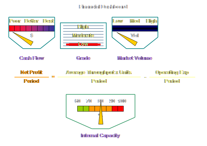
And I would like to embellish this further – or at
least make it easier for me to understand – by adding some “gauges” to this;
a sort of metaphorical dashboard for our system. And let’s assume for the moment that this
is the view prior to implementing our new-found knowledge.
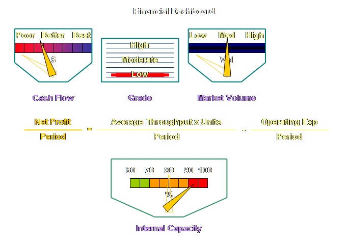
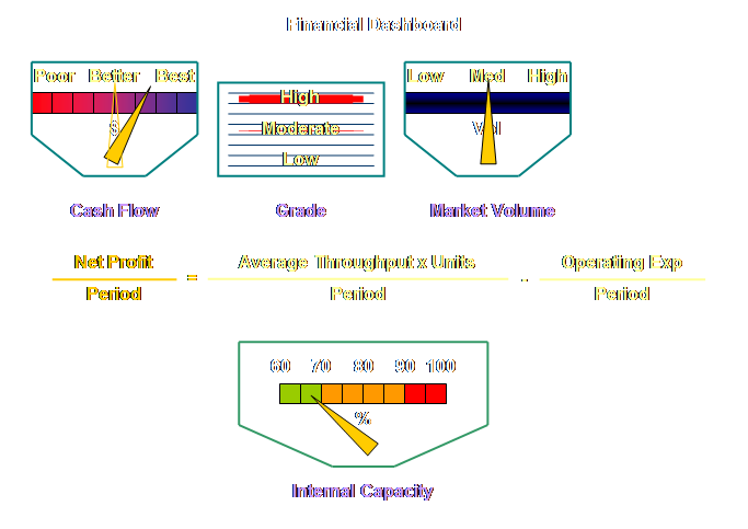
Therefore, let’s exploit this internally constrained
system and see what happens.
This is a way of showing that in an internally
constrained system it is the Throughput grade that
is most important in raising the net
profit of the system. If you can
actively substitute high grade products for low grade products in any new
orders, then you will improve your cashflow. Now a question; is this active substitution an
example of exploitation or of subordination? My answer to that is both! We further exploited the constraint (and
therefore the system as a whole) by subordinating our output decisions in
order to maximise the throughput grade.
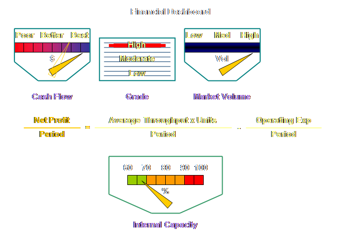
However, do we want to stay in this zone, the red zone of our constraintometer? Shouldn’t we try to bring the operation
down, or rather the capacity up, into the green zone? In essence we are beginning to tread into
an area where we need to distinguish between tactical and strategic
decisions. There is no need to tread, let’s rush headlong in! In our evaluation decisions we are essentially
asking what effect an actual action now, or a potential action in the future,
has upon our profit and/or our return on investment. These, after all, are our measures of
success in a for-profit organization.
We need to know whether the change is a significant improvement or
not, and if so, the magnitude of the improvement as well. However, we can also examine these actions from
another viewpoint – whether they are tactical or strategic in nature. I will suggest that net profit is largely a
tactical decision; how can we best maximize the return on our current
assets. Return on investment is
largely a strategic decision; how can we best maximize the return on any
additional assets. It’s not a clear
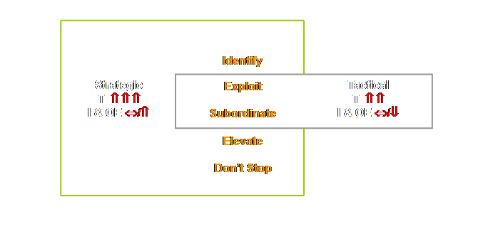
cut dichotomy, but it may be useful nevertheless. We can place this distinction within the framework
of our plan of attack, our 5 step focusing process. Let’s show the generalized effect on
throughput (T), inventory/investment (I) and operating expense (OE) within
this framework.
Let’s now consider the steps identify and
elevate. When we elevate a constraint
we most often bring additional investment into the system, usually in the
form of the purchase of additional capacity.
We may also need to increase operating expense in order to utilize the
new capacity. Thus inventory
(investment) will increase and operating expense will most likely increase
also, if only due to the increased depreciation of the new investment. Because investment is most often required
at these stages, let’s suggest that this is a strategic decision. Both tactical and strategic decisions should have a
positive impact of the productivity of the system. This is easy to determine for
non-investments. But the moment we
make an investment it is no longer straight forward. Investments are apparently invisible to our
definition of productivity;
Of course neither tactical nor strategic decisions
should be passive – determined by the next accidental emergence of a new
constraint. They should be the result
of active analysis of where we want the constraint to be. After all, the location of the constraint
dictates the way in which our firm will make money – and where our capital
investment, product development, marketing and sales efforts will be. Sometimes where there are
significant cost/capacity differences across the system we may find that the
constraint becomes by default; (1) the
most capital intensive step in the process (2) the
most capacity extensive step in the process and this is the least
likely to be overcome anytime soon because of; (1) direct
cost in the case of the most capital intensive step (2) indirect
costs of bringing up sufficient sprint capacity in the non-constraints for
the most capacity extensive step. The subdivision of whether
something is tactical or strategic based upon external investment is a useful
distinction; however, often substantial improvement can be obtained without
additional investment at all. In fact
during this tactical phase questions of strategic importance will occur. So, let’s not be mislead into believing
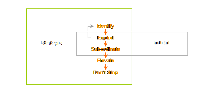
that constraints are only broken by elevation. Often, especially in the earliest stages of an
implementation, proper exploitation may be all that is required to break an
apparent constraint and to expose a new constraint somewhere else in the
system. Let’s call this an immature
stage and let’s try and draw it.
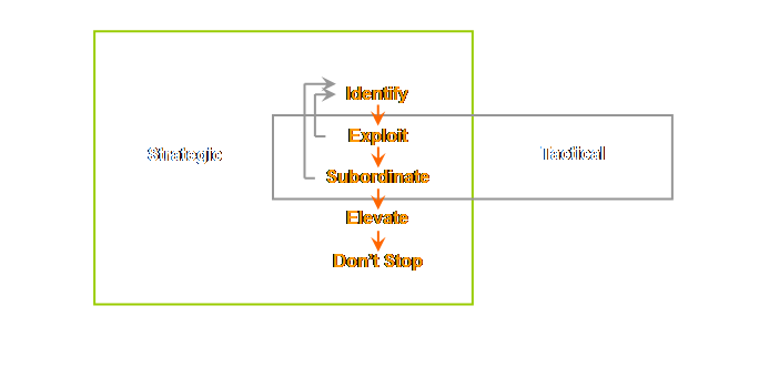
We can also break an apparent constraint simply by
proper subordination. Consider in
manufacturing where non-constraints may be regrouping separately scheduled
process batches together again – insubordination in fact (pun intended). This will actually slow the whole process
down and if it occurs in one area – maybe near the gating operation for
instance then it may manifest itself as an apparent physical constraint
somewhere else within the process. The
other extreme might be when sprint capacity is beginning to be eroded due to
increased output, constraints will appear to be “breaking out” in various
places – however the solution is to increase the buffer size. Really the constraint in both cases is in the
inertia of our subordination policies.
We can “short” the loop once again; identify-exploit-subordinate-identify.
Let’s add this.
In more mature implementations however the dynamic
is a little more constrained. In more
mature implementations there is a strong interrelationship between
exploitation of the constraint and subordination of the non-constraints. Breaking a constraint is more likely to
arise out of this interaction than either exploitation or subordination
alone. Let’s show this.
If the location of the constraint dictates the way
in which our firm will make money, or the way in which our organization will
make output, we may in fact have a preferred place for the constraint to
be. It may remain in the same place
for long periods of time; both static and strategic. Too often at first we are confused by our
prior experience and the notion that bottlenecks “wander” or “pop up.” We can control the process if we want to. In fact we must. Sometimes the methods of evaluating change are
derided as short-term by those who do not understand their strategic
significance. Sometimes too, the
focusing process, our plan of attack, is considered a short-term tactical
methodology. Both interpretations are
shallow and impoverished. There is a special richness in the focusing process
that is lost on many people – after all it is not exactly explicit about
it. Others, however, have gone to
considerable lengths to highlight this richness; often supplementing new
words into the scheme. The strategic
nature of the focusing process is important.
If you are especially comfortable with this concept, or more so if you
are especially uncomfortable with this concept, then at some time in the
future please come back for an extended discussion here. Ultimately, however, if we keep elevating our
internal constraint – even if we choose to keep it in one selected place –
then at some time we will move the constraint into the market. Many argue that this is exactly where it
should be. Theory of Constraints had its genesis in internal
capacity constrained systems. A great
deal of the early literature deals with this exclusively. Sometimes then, there is a disjoint as we
start to deal with external constraints.
I don’t believe that this disjoint exits in reality, I think that it
is symptomatic of the history and some inertia in terminology as we move out
from an internally constrained environment that is within our span of control towards an externally constrained
environment that is often only within our sphere of
influence – or so we like to think. Because we won’t touch upon this again until the
supply chain pages let’s be sure to understand that even though the constraints may now be external, the solutions are always internal.
Otherwise, how else could we ever bring about the solution? Let’s return to our see-saw analogy once again, and
continue from where we left off with an internally constrained system where
one unit of operating expense can leverage 7 units of throughput.
How then do we evaluate change in this new
circumstance? Our constraint has now
disappeared off into the market; the constraint has become nebulous rather
than physical. To answer this question we need to just slightly
reframe the situation. Sure, the
constraint is now in the market, but ask yourself, where is the internal
weakest link? It’s still back in the
physical process somewhere; most likely exactly where we last left it. Let’s have a look.
Back to our
dashboard. How has it changed since we
last left it?
However, too often this is exactly
where the disjoint occurs. You see we have two pathways down which we
can travel. The first is to increase
loading on the internal constraint.
Let’s have a look at this.
What then of the other
pathway?
Let’s have a look.
You know, we spend so
much time and effort exploiting the financial advantage of an internally
constrained system (because we have no choice) and then the moment that it
becomes externally constrained we suddenly discontinue to properly exploit
the financial advantage (because now we have a choice), and we so often
decide to accept volume instead of grade because for maybe the very first
time we can accept volume. I’m afraid that this
won’t do, not if we have a strategy. We press the issue when
we have an internal constraint that the sales people must be aligned with the
value that the constraint can produce.
We don’t waste valuable and limited constraint capacity on goods of
lower value when we can move goods of higher value, and by definition we
can. This is, after all, a central
part of our exploitation tactic. It
shouldn’t be any different when the capacity has risen to such an extent that
the constraint is now external to the system unless there are issues about
solvency. When we were internally
constrained, the grade of the earnings were paramount because in fact we
couldn’t affect the cashflow in any other meaningful way. Does this change now? Do we send our sales people out with instructions
that any additional dollar is a good dollar just because additional volume is
now an option? Heck no! We just trained them. OK “trained salesman” is an oxymoron;
rather, we just got them aligned with one set of ideals, then we throw that
out and bring in another? I don’t
think so. We are after both dimensions now, not just one or the other. We want both the best grade of Throughput
as determined the internal weakest link and the most volume of
Throughput as determined by the capacity of the external marketing
constraint. To put it bluntly; we are
after the “fat guys.”
We get them on the see-saw by changing our
policies. Our system will still
contain some policy issues that stop our customers from buying our goods;
moreover, our system will still contain some policy issues that stop our customers
from paying more for the same goods.
This is because we fail to explain to our customers (and our
salespeople) how our value delivers real additional value to them. We have to surface and remove these policy
issues. If you like, we elevate the
system by extending a policy plank, a policy extension, call it what you
like; it most probably will cost us nothing but it will substantially improve
the profitability of the organization. It seems odd to say it, but we must; we can’t
evaluate change without a strategy. It
seems odd because so often we infer that a strategy exists – our personal
interpretation of what we deem the strategy to be. However, we must make sure that we all know, understand, share, and
are aligned with the same strategy
– implicit or explicit. We simply
can’t evaluate a local tactic without knowing the overall strategic
intent. To develop this notion
further, let’s return to our analogy one last time. Remember when we had a mix of adults and children on
the see-saw, each occupying an individual position?
What if the strategy had been to develop “thrills
for mature adults?” Then surely we
might risk future success by having too many children on-board. What if the strategy had been to develop “a fun
environment for children?” Then having
too many “old” people around might equally risk future success. What if the strategy was “good value family
fun?” Then the current tactic might be
perfectly acceptable. And maybe, just
maybe, we could have protected our throughput too. Consider the following;
But the more important point is we can’t evaluate a current tactic without knowing the
strategy. And therefore we can’t
evaluate change without knowing the strategy. Sure, we started with a context, our rules of
engagement, but this is insufficient.
It is necessary to go one level deeper below
the necessary conditions and the
goal. We need to know the next layer
down, this is the first place where a "strategic intent" becomes
apparent because it is the first place where non-generic company-specific
objectives can occur. Dettmer terms
these first several layers below the goal “critical
success factors” in his Constraints Management Model for Strategy
(7). We will cover this model in more
detail in a page of its own. In a for-profit organization, regardless of whether
we are currently internally constrained or currently externally constrained,
we must ask if we will we accept any sale that has a throughput that exceeds
the raw material cost or the 1:1 variable cost? This is not a trick question. We think that we know the answer when we
are internally constrained – at least in theory – because we know how to
maximize the throughput on the constraint by adjusting the mix. But even there we have to have an eye to
the future and the overall strategy. More importantly, because the answer is less clear,
we need to know what happens in an “external” market constrained
situation. If for example our market
is constrained; we can make several sales with a low grade Throughput now,
and one sale with a high grade Throughput.
This isn’t a problem now, but it might be in the future. It might be if our market thinks that we
are a supplier of low grade Throughput goods or services. We need to ask would we knowingly forgo a
larger and on-going Throughput in the future in order to secure a smaller
Throughput now? Forget about discounted cash flow, just use common
sense. The answer is no! Well, the answer is no, unless cash is the most
important thing, which is to say that immediate solvency is such an issue
that there might be no future unless we address the “now” both quickly and
effectively. But really this is an
issue for solvency practitioners. So, accepting a low grade Throughput now for most
firms is trading short-term gains against long-term success. It is a local
optimization in time. We trade a short-term, hopefully one-off,
and local benefit for long-term, on-going, and global benefit. Why, why, why, do we do this to ourselves? We move away from local optimization in
space in our process – and to be frank we are usually overwhelmed by the
improvement – and then we completely fail to remove local optimization from
time. Why is this?
Any ideas? Could it be impatient investors? Unhelpful institutions? Our cherished Christmas bonus? Pressure from wage rounds? The local council or municipalities’ new
rate structure? Hell no, the goal of
our business isn’t to furnish cash to ever-increasing rate demands, is it? Could these be excuses? Excuses for the lack of something. Excuses for the lack of an actual strategy. Really, that is still too superficial; it is really
the lack of understanding or belief in a strategy. And we are not talking about a plan or an explicit
document – we have all seen those. We
are talking about an implicit understanding between members of the group
about where we are now and where we want to be in the future and how we are
going to get there. Once we understand the strategy, the tactics will
fall into place. Once we understand
how we intend to exploit the system, the subordination issues will fall into
place. Moreover, once we have a
strategy then having a unitary internal constraint makes a world of
sense. Where the constraint resides is
no longer an issue. We may modify our
actions accordingly but the path is understood by all. Now, finally, we are in a position to explain and
understand a conundrum that usually hooks people up and doesn’t let go – the
dilemma arising out of subordination of the local to the global. The dilemma is expressed at two levels, here is the
first. We must subordinate the current tactical constraint to the future strategic constraint. Consider for example a tactical constraint that is
the paint booth in a small engineering shop, and we want the constraint to
eventually move to the assembly area of that shop. In order to do so, we may have to forgo
maximum financial throughput per unit time on the current tactical constraint
in order to build the correct business for the future desired financial
throughput on the chosen strategic constraint. We can step this out, here is the second level. We must subordinate the current strategic constraint to the future strategic constraint. We can see exactly this in Toyota today as that
company develops hybrid engine technology and brings it to market ahead of
perceived demand (8). The development
of the Cummins Engine Company and the philosophy of the Irwin-Sweeny-Miller
families is another exceptional example of this process (9). Both of these firms leverage on the present
to create the future. The leveraging
results in lower current profit than would otherwise be possible and a
greater future (and total) profit than would otherwise be possible. In fact, we could step back a little to
contemplate how Toyoda Spinning and Weaving – a very successful firm in its
own right, chose to, and evolved into an auto manufacturer. Caspari and Caspari capture this dilemma which
occurs whenever such a new strategic constraint is selected. The dilemma is presented very nicely as a
short-run versus long-run cloud (10). Generically it looks like this;
A conflict arises, however, from the extension of
these needs. In order to have good
tactics we must exploit the current constraint. But, also in order to have good strategy we
must move the system towards the future desired strategic constraint –
otherwise our leadership decisions will not be implemented. And herein lies the dilemma; we can not
both exploit the current constraint and not exploit the current constraint
(move the system towards the strategic constraint). How can we break this dilemma? Let’s see.
In fact, if we substitute “long-run”
for “good strategy” and “short-run” for “good tactics,” then we can clearly
see the relationships.
We must not locally optimize in time – unless we are
willing to sub-optimize globally over a longer period. Moreover, our short-term results only have
significance with respect to our overall strategy. If there is no strategy then short-term
gains will be overwhelmingly attractive.
If there is a strategy and the strategy is understood by all, then the
future gains will be far more attractive. Subordination remains the key; we must subordinate
the non-constraints to the constraint of the system and we must subordinate
the tactics to the strategy of the system.
This requires good leadership. Robert Simons in Levers of Control
wrote about the need to establish a critical bridge between the disciplines
of strategy, accounting, and control (11).
He did so using 4 systems as his levers. We can extend his analogy from levers of
control to levers of profit in for-profit organizations, and levers of
success in for-cause organizations. The terms “levers of profit” and “levers of success”
highlight that we leverage the system via a constraint in the physical
system. We can leverage the system by
changes in investment and expenditure, but more importantly we can also
leverage the system by changes in policy.
In the end it is really people who offer the real leverage in these
man-made systems. Regardless of how we
leverage the system we must not forget that the fulcrum “under” the lever is
time.
We can make a quick and stunningly effective
evaluation of changes that are improvements by taking care to use the 3
fundamental measurements of throughput, inventory/investment, and operating
expense while remaining mindful of where the pivot point and the constraint
are now and indeed where we would like them to be in the future. Let’s turn our attention now to some of the broader aspects,
aspects that make all of this happen; aspects of leadership. This page supersedes one initially entitled “accounting for change,” which is included here as a
link as it is still referenced by a number of other pages. Rather than use this link, there are two
excellent sources for accounting professionals. They are; Caspari, J.
A., and Caspari, P., (2004) Management Dynamics: merging constraints
accounting to drive improvement. John
Wiley & Sons Inc., 327 pp. Corbett, T.,
(1998) Throughput Accounting: TOC’s management accounting system. North River Press, 174 pp. I originally
wrote this page because I wanted to address evaluating change without recourse
to equations – well at least not straight away. This was the rationale for the see-saw
analogy. But there was another
motive. I was “irked” that the texts
said that once we move from internally constrained to externally constrained
“any additional cash will do.” I was
concerned that if you are going to invest cash on a project then your really
want the best grade return that you can obtain – even if you have to wait a
while. Moreover, when
I wrote the original version of this page Viable Vision was little known and
even less understood. Yet the heart of
Viable Vision is exactly the high grade exploitation of the external
market. I’m sure that as the text
books arrive at new editions this necessary condition of maximising
throughput in externally constrained systems will be much better explained. Of course
Viable Vision aims at turning the top line (annual sales) into the bottom
line (net profit) in 4 years. This
seems unbelievable, but it is all a matter of strategy. If we have mediocre expectations and
mediocre strategy, then we will get mediocre results. If we have a strategy that is staged around
the breaking of a sequence of internal and external constraints while all the
time seeking high grade throughput then Viable Vision in various environments
is an absolute reality. (1) Goldratt, E. M., (1990) The haystack syndrome: sifting
information out of the data ocean.
North River Press, pg 98. (2) Goldratt, E. M., (1990) The haystack syndrome: sifting
information out of the data ocean.
North River Press, pp 96-97. (3) Caspari, J. A., and Caspari, P., (2004) Management Dynamics: merging constraints accounting to drive improvement. John Wiley & Sons Inc., pp 115, 118-119. (4) Corbett,
T., (1998) Throughput Accounting: TOC’s management accounting system. North River Press, pg 55. (5) Schragenheim, E., and Dettmer, H. W., (2000)
Manufacturing at warp speed: optimizing supply chain financial
performance. The St. Lucie Press, pg
240. (6) Caspari, J. A., and Caspari, P., (2004) Management
Dynamics: merging constraints accounting to drive improvement. John Wiley & Sons Inc., 327 pp. (7) Dettmer,
H. W., (2003) Strategic navigation: a systems approach to business
strategy. ASQ Quality Press, 302 pp. (8) Liker, J. K., (2004) The Toyota Way: 14
management principles from the world’s greatest manufacturer. McGraw-Hill, pp 71-84. (9) Cruikshank, J. L., and Sicilia, D. B., (1997)
The engine that could: 75 years of values-driven change at Cummins Engine
Company. Harvard Business School Press,
587 pp. (10) Caspari,
J. A., and Caspari, P., (2004) Management Dynamics: merging constraints
accounting to drive improvement. John
Wiley & Sons Inc., pp 261-262. (11) Simons, R., (1995) Levers of control: how
managers use innovative control systems to drive strategic renewal. Harvard Business School Press, 215 pp. This Webpage Copyright © 2005-2009
by Dr K. J. Youngman |