|
A Guide to Implementing the Theory of
Constraints (TOC) |
|||||
|
A Motor For Production Drum-buffer-rope is the Theory of Constraints
production application. It is named
after the 3 essential elements of the solution; the drum or constraint or
weakest link, the buffer or material release duration, and the rope or
release timing. The aim of the
solution is to protect the weakest link in the system, and therefore the
system as a whole, against process dependency and variation and thus maximize
the systems’ overall effectiveness.
The outcome is a robust and dependable process that will allow us to
produce more, with less inventory, less rework/defects, and better on-time
delivery – always. Drum-buffer-rope however is really just one part of
a two part act. We need both parts to
make a really good show. If
drum-buffer-rope is the motor for production, then buffer management is the
monitor. Buffer management is the second
part of this two part act. We use
buffer management to guide the way in which we tune the motor for peak
performance. In the older notion of planning and control, the
first part; drum-buffer-rope, is the planning stage of the approach –
essentially the overall agreement on how we operate the system. The second part, buffer management, is the
control system that allows us to keep a running check on the system
effectiveness. However, I want to
reserve the word “planning” and the word “control” for quite specific and
established functions within the solution, functions that we will investigate
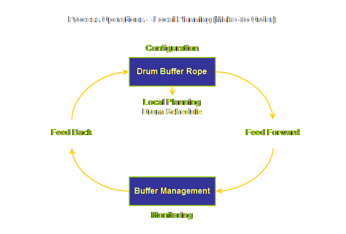
further on this page. I want to propose that we step out
a level and instead use the terms “configuration” and “monitoring.” Using this terminology the configuration is
drum-buffer-rope and the monitoring is buffer management. Let’s draw this;
Keep this model in mind as we will return to
it. Now, however, we must return to
our plan of attack and work through the development of the solution. Interested?
Then let’s go. On the measurements page we introduced the concept
of our “rules of engagement” which is to define; the system, the goal, the
necessary conditions, the fundamental measurements, and the role of the
constraints. Then on the process of
change page we introduced the concept of our “plan of attack” – the 5
focusing steps that allow us to define the role of the constraints. Let’s remind ourselves once again of the 5
focusing steps for determining the process of change; (1) Identify the system’s constraints. (2) Decide how to Exploit the system’s constraints. (3) Subordinate everything else
to the above decisions. (4) Elevate the system’s constraints. (5) If in the previous steps a constraint has been broken Go back to step 1, but do not allow inertia to cause a system
constraint. In other words; Don’t
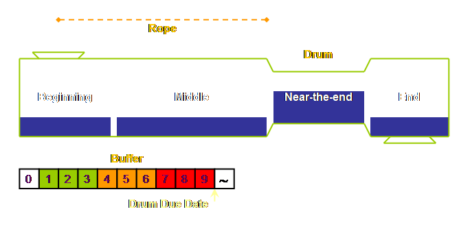
Stop. Let’s also return to our simple system model which
we have so far used in much more general terms and apply it to
drum-buffer-rope. As you will recall
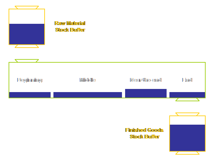
it has 4 sections, or departments or whatever you would like to call them; a
beginning, a middle, a near-the-end, and an end.
In fact we know where the constraint is in our
simple system presented here based upon the discussion in the earlier section
on measurements. It’s located near the
end of the process. This isn’t at all
an unusual place to find a constraint.
Think about it for a moment. If
the constraint was located near the beginning, then all the downstream steps
would always be waiting for work. In
that situation management would most probably go about purchasing further
capacity until they move the constraint further down the process and then
bury it in work-in-process so that it is no longer visible. Let’s draw the constraint in.
Of course we forgot something –
work-in-process. If our model system
is to be anything like our own reality, then it is probably full to the gills
of work-in-process. We had better add
this to our model as well.
So we have completed Step 1 – identify the
constraint. The next step, step two,
is to decide how to exploit the constraint. To make sure that the constraint works as well as
possible on the task of producing or creating throughput for the system we
must ensure that we exploit it fully – essentially we are leveraging the
system against the full capacity of the constraint. This means not only making sure that it is
fully utilized, but also making sure that the utilization is fully
profitable. If you remember back to
the P & Q problem or the airline analogy, is quite possible to have
everything utilized but not make as much profit as is possible. If we increase the output of the
constraint, then the output of the system as a whole will increase also. One of the most effective tactics for
exploiting the constraint, once identified, and improving its output is to
write a detailed schedule for that particular resource and that particular
resource alone – and then to adhere to that schedule. This is the “plan” in this context. Our day-to-day planning “falls out” as a
consequence of the decisions that we make while configuring the
implementation. Let’s add this to our
model.
If we continue to operate in this fashion we can
reduce work-in-process considerably.
Let’s show this before introducing some further drum-buffer-rope
concepts.
Sometimes using the word “protect” makes it easier
to understand this step than using the correct term which is
“subordinate.” In fact, we subordinate
the non-constraint resources in order to protect the constraint and
the system as a whole. Let’s examine
this is a little more detail. In the process of change page we described
subordination as avoiding deviation from our plan, and the plan in this case
is our constraint exploitation schedule in the previous step. We described deviation from plan as (2); (1) Not doing what is supposed to
be done. (2) Doing
what is not supposed to be done. We can therefore describe subordination as; (1) Doing
what is supposed to be done. (2) Not doing what is not supposed
to be done. By doing what is supposed to be done in accordance
with our plan we protect the constraint and the systems as a whole. Moreover, by not doing what is not supposed
to be done in accordance with our plan we also protect the constraint and the
system as a whole. Let’s examine this
with our simple model. As we use up our supply of excess work-in-process,
it is likely that the constraints will begin to “starve” from time to
time. Work will not arrive in
sufficient time for it to enter the constraint on schedule. We need to replace our local safety everywhere
(our excess work-in-process) with some global safety right where it is
needed, in front of the constraint. We
need to buffer the constraint. We need to do what is
supposed to be done in order to protect
the constraint from shortages. In fact we would normally have made our buffering
decisions before we even began and therefore reduced our work-in-process and
lead time in line with these pre-determined targets. Let’s assume for a moment then that the lead time
allowed for work to travel from the start of the process to the start of the
constraint was 18 days prior to the implementation. Well, in fact, it could be 18 hours for
electronics or the paper work in an insurance claim, or it might be 18 weeks
for heavy engineering. But let’s use
days in this example. The rule of
thumb to apply is to halve the existing lead time (3). Therefore the new lead time becomes 9
days. If halving the lead time sounds
horrendously short, it is not. Most of
the time the current work-in-process is sitting in queues doing nothing. You can easily check this for yourself –
got out and tag some work with a flag or a balloon or a bright color and then
watch it. It will sit. This 9 day period becomes our buffer
length. To this 9 day buffer we apply a second rule of thumb
and divide the buffer into zones of one third each (4). We expect most work to be completed in the
first 2 thirds and be waiting in front of the constraint for the last third
of the buffer time. Thus we expect our
work to take about 6 days of processing (and waiting-in-process) and 3 days
of sitting in front of the drum. If 3 days sitting in front of the constraint sounds
terrible, then remember that prior to
the implementation, the system allowed work to sit for at least another 9
days. Nine plus 3 is 12 days
sitting. Which would you rather have
12 days or 3 days? More importantly,
which would your customer prefer? We now can protect our system constraint by ensuring
that there is always work for it to do.
Thus we ensure its effective exploitation – and with much less total
material or lead time than before. Let’s add the buffer to our diagram.
Please be careful, on the diagram above we have
drawn units of time – the zones and the buffer – as space on our
diagram. Don’t let this confuse
you. The zones equate to time allocated
in the plant to protecting an operation whose position and function is
critical to the timeliness and output of the whole process. The zones do not equate to the position of
work in the plant. In fact we will
return to this shortly and try and draw the diagram more realistically to
represent time. Why is this whole period from material release to
the constraint considered as the buffer?
Schragenheim and Dettmer consider that this is one of two unique
aspects of buffering in Theory of Constraints. “The reason buffers are defined as the
whole lead time and not just the safety portion is that in most manufacturing
environments there is a huge difference between the sum of the net processing
times and the total lead time. When we
review the net processing time of most products, we find it takes between
several minutes and an hour per unit.
But the lead time may be several weeks, and even in the best
environments several days.
Consequently, each unit of product waits for attention somewhere on
the shop floor for a much longer time than it actually takes to work on
it.” “So it makes sense not to isolate
the net processing time, but to treat the whole lead time as a buffer – the
time the shop floor needs to handle all the orders it must process (6).” The other unique point is that buffers are, as we
have mentioned, measured in time.
Firms in non-drum-buffer-rope settings consider a buffer to be a
measure of physical stock; 6 jobs, or 6 orders, or 10 batches, or 4000
pieces, or whatever. In
drum-buffer-rope a constraint buffer is a measure of time; hours or days of
work at the constraint rate located between the gating operation (material
release) and the constraint. In fact,
there are two ways to look at a buffer, either from the perspective of a
single job, or from the perspective of the system as a whole. Let’s consider this for a moment. Let’s assume for the sake of simplicity that all of
our jobs are of equal length. Let’s
assume then that each one takes 1 day of constraint time. In this case each job has a 9 day buffer to
the constraint. That is, it is
released 9 days prior to its scheduled date on the constraint. This is the perspective of a single
job. The constraint, looking back,
will see 9 one-day jobs at various stages in the process; this is the
perspective of the system as a whole. What then, all else being equal, if all of our jobs
now take half a day on the constraint?
Each job sees a 9 day buffer, the constraint looking back will see 18
half-day jobs at various stages in the process, but the aggregate load is still
9 days, this is the perspective of the system as a whole. Let’s do this one more time. Each job now takes quarter of a day on the
constraint. Each job still sees a 9
day buffer, the constraint looking back will see 36 quarter-day jobs at
various stages in the process, but the aggregate load is still 9 days from
the perspective of the system as a whole.
It is time that is the measure of the buffer. Let’s labor this point for a moment because it is so
important. Measuring a constraint
buffer in units of time is unique to drum-buffer-rope because acknowledgement
of the existence of a singular constraint within a process is unique to
drum-buffer-rope. We can apply this to
both the constraint buffer size and the constraint buffer activity. Let’s look at constraint buffer activity first. By considering only one station, or step, or
procedure, we need only to know one set of average times for that place or
action for all of the different types of material units that pass through
it. We could look at this as follows; At a manufacturing constraint an hour is
an hour but the number of units may differ The number of physical units may differ because
different types of material using the same constraint may use different
amounts of constraint time. In fact,
even the same type of material will display some variability unless the
constraint is a totally automated procedure – but these will largely average
out. How about constraint buffer size then? The unique perspective brought about by the
designation of a singular constraint allows us to define the length of the
buffer in time also. Essentially the
buffer is sized and “sees” the duration from the gating operation to the
constraint due date. Moreover the
buffer “sees” committed demand – work that has already been released
to the system. Constraint buffers,
divergent/convergent control point buffers, assembly buffers, and shipping
buffers are all of the same basic nature. Maybe it is much simpler to say that; We protect time (due date) with a time buffer There is, however, one other buffer type that we are
likely to come across in manufacturing – a stock buffer. There are two places that these occur at in
manufacturing; they are at raw material/inwards goods in all process
environments and at finished goods in a make-to-stock environment. These are actually supply chain buffers;
they represent the two places that the supply chain must interact with processing
– before the beginning of the process and after the completion of the
process. We need to ensure that we
always have an adequate supply of raw material prior to the process to meet
consumption and we need to ensure that we always have an adequate supply of
finished goods post-production to meet demand. We will examine these types of buffers
later on this page. They are also
examined in more detail on the supply chain pages – especially the
replenishment page. However, let’s
confine ourselves at the moment to constraint buffers. We need to labor the issue that the
constraint buffer is a measure of time.
Let’s do that. Many, many, people say that they do understand the definition of a drum buffer or of a
constraint buffer when the evidence is that they do not. Too often our prior experience causes us to
think of buffers in terms of physical stock, and too often we consider zone 1
as “the buffer.” Let’s see.
In part, this is due to our prior manufacturing
experience with MRP II systems and push production which tends to blind-side
our interpretation (see the sections on Buffer The Constraint and Local
Safety Argument in the next page – Implementation Details – for further development
of this aspect.) In part, the problem
also lies in the way we try to draw time as space on our simple diagrammatic
representations. The only way to draw
time is to draw a sequence of diagrams.
Let’s do that. We will follow a slice of work – ones day’s worth –
through the process to the drum. We
will use our 9 day buffer as we derived above, so this slice of work is the
drum’s work for one day 10 days out from the scheduled processing date. There are 5 products (units, jobs, batches,
whatever) in our slice. The products
are “lilac,” “red,” “green,” blue,” and “orange.” The time interval, for the sake of clarity
in this example, is course – days – rather than finer divisions of hours or
less that we might expect to find in reality. Imagine that within the departments (“beginning” and
“middle”) of our generic process we have the tools of our particular trade;
be they desks in a paper trail, admission or beds or clinical units in a
hospital, or work centers in a manufacturing system. The 5 products could be at any time waiting
or moving between jobs or being worked upon.
The resolution of this detail isn’t important to us here. Probably in the day before the release date the
planner knows what will be released.
The planner might even have the orders “cut” and waiting but
unreleased (and hopefully unknown to the floor – to avoid people working
ahead of time). Let’s draw this.
We have also drawn a timeline in. It is colored according the buffer
zones. Zone 3 is the “green zone,”
zone 2 is the “orange or yellow zone,” and zone 1 is the “red zone.” On the first day of the schedule all the products
are released (as scheduled) and are in zone 3 of our time buffer. Their physical location at the end of the
day is as follows.
After another day we are at day 2 and still within
buffer zone 3 the process looks like this.
By day 4, one day into buffer zone 2 we see the work
has evolved as follows.
The next day, day 5 (buffer zone 2), the work looks
like this.
At the end of day 6 – the last day of buffer zone 2
we see the following.
Let’s go out to the end of day 7 and see what
happens.
Let’s now look at the situation at day 8.
So, let’s reiterate once more; buffer zones equate
to the time allocated in the plant to protecting operations whose position
and function are critical to the timeliness and output of the whole process, buffer
zones do not represent the physical location of work in the plant. We know how to protect the constraint, now let’s see
how to protect everything else. So, we know now how to protect the constraint using
a buffer, we therefore know how to do the first part of subordination – doing
what we are supposed to do in order to protect the constraint. Now we need to examine the second part of
subordination – not doing what we are not supposed to do. First, let’s repeat the diagram that we first drew
prior to our journey along the buffer.
In order to maintain stability in this system, the
rate at which the gating operation allows the admission of new work to the
system must be the same as the rate of consumption at the drum. What would happen then if our constraint
breaks down for a short period? It has
no spare capacity, so we can’t speed it up (allow it to work longer) to catch
up to the work again. If we were to
continue to admit work as though nothing had happened then work-in-process
would increase a little. Probably not
enough to notice, but over a couple of different instances it would begin to
build up. Thus we need to make sure
that we admit new work into the system at the same rate as the constraint is
consuming it. The constraint as we
know is the “drum” of our system, beating out the rate at which the whole
system works, including the gating operation.
The rate is communicated to the gating, or first, operation by the
“rope.” We need to add this to our
diagram. If you like, the schedule of the gating operation is
the schedule of the drum off-set by a rope length of time. The rope length is the same as the buffer
duration; the gating rate is the same as the drum rate. “Tying” the rope between the drum and the
gating operation ensures that excess work can not be admitted, or that normal
work can not be admitted too soon. This
is part of not doing what is not supposed to be done
in order to protect the system from excess
work-in-process. Excess work in
process results in longer than necessary lead times and poorer quality. Ultimately excess work-in-process also
impacts upon the throughput of the constraint. Another way of looking at the rope is to consider it
as a real time feedback loop between the drum and the gating operation. Although the constraint can not recover from
down-time, hence the need to exploit and protect it, the non-constraints can
recover from down-time. Generally the
non-constraint parts of our system don’t work at the same rate as the whole
system – at least over short periods of time.
The non-constraints have sprint capacity. They can and do process more work when
necessary to catch-up after a “bump” in the system by operating at normal
rates for longer periods. They can
also process less work when not needed by operating at normal rates for
shorter periods. We might consider the increased duration of
non-constraint processing (in order to catch up) as the “doing what is
necessary” part of subordination, and the reduced duration of non-constraint
processing (to avoid over-production) as the “not doing what is not
necessary” part of subordination. It
is critically important that we do this. In the Toyota production system, kanban perform both
of these functions. In
drum-buffer-rope this is performed by the “roadrunner” concept. When we have work to do, we do it. When we don’t have work to do, we don’t do
it. We saw this in the form of the
traffic light analogy earlier in the page for process of change. Non-constraints should never “slow down,”
they should either be fully-on or fully-off (maybe that should be normally-on
or normally-off). Either creating
throughput or protecting throughput.
We will revisit this theme on the next page; implementation details. We have seen how we now have 9 days of work in
process in our example – down from the initial 18 days. There are 6 days of work in process in
zones 3 and 2 and three days in zone 1.
But we can think about it in another way. By halving the work-in-process we have
removed 3/6ths of the work from the system.
We have another 1/6th sitting in front of the constraint, so in effect
we have just 2/6ths or 1/3rd of our previous work-in-process actually on the
floor being actively worked on or sitting in queues. Imagine your process at it stands today but
with just 1/3rd of the work actively being worked on by the non-constraints
or waiting-in-process; wouldn’t things really begin to flow in that
situation? Nevertheless, in order for that material to flow, it
is critically important to protect sprint capacity by proper
subordination. Sprint capacity
interacts with overall buffer size and hence manufacturing lead time. We will investigate sprint capacity more in
the next section. Protecting sprint
capacity means that we never admit work into the process just to keep people
busy – never. Of course you will have noticed that we have so far
used the departmentalized version of our system model. To some extent this was intentional because
when you first approach a drum-buffer-rope implementation, the process will
be departmentalized. However, what we
would like to see after a short while is a better appreciation of the system
as a whole. Conceptually it should look more like this;
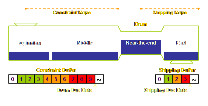
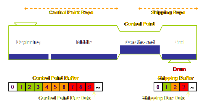
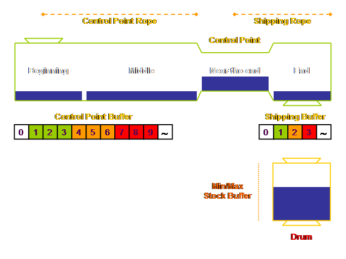
For the shipping buffer, we again apply the same
rules of thumb as we used for the constraint buffer. Let’s assume, for the sake of the ease of
the mathematics, that the process downstream from the constraint to shipping
currently takes 6 days. We halve that
to give us a new lead time of 3 days.
And then we divide that into buffer zones of thirds and expect almost
all work to be completed after 2 days and either waiting for shipment or
already shipped 1 day prior to the shipping date. This is what we arrive at;
Thus our original 24 day process becomes a quoted
delivery time of 12 days. The system
should be able to produce more because we will have made every effort to
exploit the constraint, and the non-constraints only work on material that is
required to support the constraint schedule. So, to summarize, subordination is the instruction
to the non-constraints. It has two
main components. Firstly; in order to protect the system as a whole
we must not starve the constraint – we must not underload
the system. This will ensure maximal
output as per the exploitation strategy of the constraint. Of course we could make the buffer quite
large and never have to worry about starving the constraint, but that is
where most systems are today (and they still starve the constraint). So we need to do something else as
well. Secondly; in order to protect
the system as a whole we must not flood the non-constraints – we must not overload the system. This will ensure adequate sprint capacity
to ensure maximal output as per the exploitation strategy of the constraint
and high due date performance. It will
also ensure a much reduced lead time. Thus we have covered all three aspects; the drum,
the buffer, and the rope. We have also
covered the first three steps of the 5 focusing steps; identify, exploit, and
subordinate. If we have fully exploited the leverage point, and
subordinated everything else, then the next thing to do is to elevate the
constraint. But first, let’s examine
an alternative initial buffer sizing rule. So far we determined our initial buffer sizes by
taking 50% of the existing lead time over the part of the system that we
wished to protect. There is another
lesser-known rule that we can also use.
We can take 3 times the back-to-back time for a job to transverse that
part of the system that we wish to protect. From time to time jobs are expedited for a number of
reasons, therefore people will know from direct experience, or will have good
intuition, for the back-to-back time and from that a buffer duration can be
obtained. Elevation may require that some additional
investment be made to purchase additional capacity that will produce
additional throughput, preferably at more than pro-rata. Remember we are trying to decouple
throughput from operating expense thereby driving productivity and
profitability up;
If at any time a constraint is broken then we must
look for the next constraint. In fact
we should know from buffer management where it will be before we even get
there. However, many times an initial
physical constraint is broken and a policy issue takes its place. Goldratt’s admonishment not to let inertia
become a system constraint is a plea to look at which policies block us from
moving forward even further. Really
this is a plea to Don’t Stop! There are a few traps for those of us who are new
players. Some of the definitions have
changed over time. In this case to be
forewarned is to be forearmed, let’s do that.
Here we have used the term “drum” to describe the entity that
determines the rate at which the whole system works – be that an internal
constraint, or as we will see, an external market demand. However the term “drum” is also used to
describe the drum schedule, in fact some insist that the drum is the schedule.
Clearly when the constraint is in the market this definition makes
more sense. Both are in use, some
would argue that these different definitions are simply different manifestations
of the same concept. If we accept
this, then that ought to keep everyone happy. Likewise, the “rope” has been used here to describe
the off-set between the drum and the gating process; however, it too is
subject to a more restrictive definition of the “gating schedule.” Once again these are different
manifestations of the same concept.
They are not mission critical. We have so far examined the development of the
drum-buffer-rope solution – our motor for production – and we have done that
within the framework of our 5 step focusing process. We also presented a model for the
configuration and monitoring of this solution, to this we have added a local
planning aspect; our schedule for the exploitation of the drum. Let’s repeat the model here and note that
we are looking at the specific case of make-to-order.
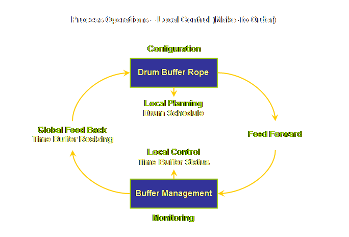
(1) Local
Control; the day-to-day exception reporting that indicates when there may be
a potential due date violation. (2) Global
Feedback; longer term trend-reporting that suggests a particular buffer needs
to be resized to be fully effective. Buffer management is crucial; it filters important
signals from the day-to-day noise of the system thereby alerting us to
potential problems before they become real problems and it provides a
self-diagnosis that neither too much and nor too little protection is made
available for each case. The self-diagnosis
feeds back into our configuration and guides improvements in the overall
dynamics of the implementation. Let’s modify our model to incorporate this.
“A reactive mechanism
that handles uncertainty by monitoring information that indicates a
threatening situation and taking appropriate corrective action before the
threat is realized.” The subdivision of buffer management into local
control and global feedback will, I hope, make it easier to understand this
important concept. Let’s now investigate the various stages of local
control and then global feedback in a make-to-order environment. We release work a rope length ahead of the due date
at the point that the buffer protects.
In most cases that is more than sufficient to insure that the work
arrives in good time. But as we know
sometimes stuff happens. We need some
local control to ensure that when stuff does happen we know the correct
priority to return the system to one of stability. We need to know the status of the current
make-to-order work orders that are already released to the system to be
worked upon. Schragenheim defines the buffer status as follows
(8); Buffer Status = (Buffer Duration – Remaining
Duration) / Buffer Duration The buffer status is synonymous with buffer
consumption. Let’s look at an example. Here we have the buffer status for 6 jobs
due in the next 5 days.
Of the current jobs; job 6 with a buffer status of
44% is no problem, we should leave it alone.
However jobs 2 & 4 both have a buffer status of 66% or more. They have both begun to penetrate zone 1 of
the buffer, the red zone. Of the two,
which is the greater priority? Clearly
it is job 2; this is the one with the greater buffer status value and is the
one that we should first concentrate our attention on. Thus the buffer status drives the work order status
once the job has been released to the system.
We therefore have local control by exception in order to meet our
global objectives. Buffer status is
viewed from the perspective of a single job. What then, where we have short ropes and long ropes,
surely that is more complicated? Again
the buffer status allows the direct comparison of work orders that have
differing buffer lengths within the same process. Let’s have a look.
Don’t confuse short jobs and long jobs with “rush”
and “standard” orders. That particular
prioritization takes place in the order queue and not in the manufacturing
lead time. In a make-to-order system where there is a
commitment to meet a due date, then; Current Work Order Status = Buffer Status It may seem redundant to state this, however, it
will become clearer when we deal with make-to-stock. In a make-to-stock environment the stock
order status can vary over time due to the natural variability of the process
itself and due to changing market demand as well. This additional factor is absent from the
make-to-order environment, here we have a commitment and we must meet that
commitment. Ever been in the situation where you have a nice
workable schedule – all the critical areas have been satisfied (all the
“squeaky wheels” are oiled), and then someone announces “you know the
material that they said would be on the truck this morning, well its not!” What are you
going to do? This job is down for the
gating operation this morning, you don’t have it, and it’s the Friday before
a long weekend. Sound improbable? Not at all. Officially you can wait. You can wait until up to 50% of the buffer
to the next stage has been consumed.
Until then the work can still be released, after that it must be
rescheduled. In fact the same logic can be applied when
back-scheduling from the shipping date.
Sometimes commitment to different customers and/or varying rope
lengths will result in a conflict where more than one job simultaneously
requires the constrained resource. One
solution is to start some work on the constraint even earlier than
required. If a conflict still exists
then some work may have to start later than we would like, in effect the late
start pushes that job out so that it begins to consume part of its shipping
buffer. Again, so long as not more
than 50% of the shipping buffer is consumed then the job can proceed,
otherwise the commitment to the client must be renegotiated – the due date
must be pushed out further (9). Stepping back one step further, the same logic
applies in-turn when back-scheduling from the drum date to material release,
now for a different reason than material lateness; we can apply the same
rules as before. In fact, this is
really local planning rather than local control, but it is easier to
understand now rather than earlier. We want to insulate our customers from the
variability and dependency within our system.
We can do this in two ways; (a) proper subordination so that
non-constraints have adequate sprint capacity, and (b) buffering so that even
when sprint capacity is exhausted for what ever reason (stuff sometimes
happens) we still have some safety time up our sleeves. Of course, we have “rolled-up” our local
safety everywhere into a few discrete and critical places where it will be of
maximal benefit. Work order status – our buffer status – tells us in
real time when to facilitate an order, and in what priority we should do so
if more than one work order requires facilitation at the same time. It is local, immediate, and
pre-emptive. A buffer status that
exceeds 66% has consumed more than 2/3rds of its buffer capacity, colloquially
we say that it has penetrated the red zone. Until the order is complete and at the buffer origin
we don’t know to what “depth” the red zone has been penetrated. However, once the order is complete and the
degree of penetration is known we can call this degree of penetration a
“buffer hole.” Let’s draw this.
What then is an acceptable frequency for buffer hole
occurrence? Well that depends. In a relative sense buffer holes should
neither be too frequent nor should they be too rare (8). A more concrete suggestion is something
less than 10% (11). Clearly the zone 1
buffer hole operates in only a limited number of cases. It is a fine example of exception
reporting. After all we want a robust
system, not one that must be pampered every hour of the day. If we take our example of a 9 day constraint buffer
we would expect most jobs to be completed before 6 days and to be waiting at
the constraint 3 days prior to their scheduled operating date. Of the remaining few we must go and look
for them in the prior operations to ensure that they will reach the constraint
before their scheduled operating date there.
If we then look at aggregate data for, let’s say 25 jobs with roughly
a 5% level of buffer hole occurrence, then that data might look something
like this;
Buffer holes are viewed from the perspective of the
system as a whole. From the buffer hole data we can construct a more
meaningful measure. In the
measurements section we discussed two local performance measures; unit days
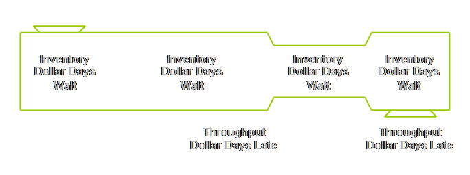
late and unit days wait. In a
for-profit environment these are known as throughput-dollar-days (late) and
inventory-dollar-days (wait). I prefer
to add “late” and “wait” to these measures because to those who are
unfamiliar with the terms it is hard to know what they mean or their
significance. And these two measures
are so important to the overall success of drum-buffer-rope that we can’t
afford to lose people through obscure terminology.
Now let’s consider the other side of the equation –
inventory. Have you ever had material
go to the outsourcers that seemed to have a life of its own – I mean it
didn’t seem to want to come back. “I
know we said this week, but one of the guys is off and now it will be next
week”. Even small jobs at the
outsourcer can have major implications if it stops an otherwise completed job
from being shipped. Of course we will
pick that up in our buffer holes and in terms of the measure of
throughput-dollar-days late. However,
sometimes, the response is to add some additional just-in-case work to guard
against this in the future. Sometimes
people will also admit new work in order to keep a particular center
“busy.” Sometimes the post-constraint
areas aren’t always diligent about keeping work moving. We can guard against these types of incidences
with our other local measure inventory-dollar-days
wait. Adding or building
work that may still be on-time is effectively captured with this
measure. Moreover it can be applied to
sub-sections of the whole process. It
helps to stop the squirrels in the business from storing inventory
just-in-case. Throughput-dollar-days late and
inventory-dollar-days wait are the two measures that effectively allow us to
monitor the stability of the system, they are local measures with
implications for global feedback. Just
two measures. You couldn’t wish for
better could you? OK, one measure,
some people can’t be pleased, but we will have to suffer two. If buffer holes begin to occur in the red zone
significantly more frequently, or indeed less frequently, than our target
level, we must do one of two things; (1) adjust the buffer or (2) adjust the
sprint capacity. Of the two, adjusting
the buffer is the most rapid and easy to do.
We simply change a policy on buffer size and accept a small
increase/decrease in total work-in-process and manufacturing lead time. We can also use the equivalent unit-day
late measure to monitor this need. If a buffer hole trend begins to “emerge” but is not
yet too troublesome, then it may indicate the erosion of sprint capacity in
the system and the area of that erosion, or it may indicate some special
cause – a machine or quality or operating problem. The cause should be tracked down,
monitored, and rectified if possible.
There are definitely cases where buffer holes arise from some
innocuous change in the process, “we used a different glue because it was
cheaper,” which has a downstream impact that was not anticipated, “yes but we
are spending more time on removing glue marks.” Emergent buffer holes also indicate
potential future constraint points. We
will investigate these factors in more detail in the page on implementation
details. Buffer management is the monitoring aspect of our
implementation and monitoring model.
It provides both local control and maybe more importantly a global
level feedback into our drum-buffer-rope basic configuration. We only “tune” the basic parameters when
the system behavior tells us that we need to do so. We only do what we should do, and we don’t
do what we shouldn’t do. If we continue to apply our plan of attack, our 5
focusing steps, then it is unavoidable that at some stage we will elevate our
system constraint so that it moves to the market. What are we going to do then? Let’s see. If the bottleneck to the system is the market, then
we must treat the market as the constraint and subordinate the process
constraint (now best called a control point) to the market. This means only making things that the
market needs and not making the things that the market doesn’t need
(overproduction). Essentially the drum
is now in the market place, but we can visualize this by placing the drum at
dispatch – the customers’ desired due date.
You see, the control point, our internal weakest
link, isn’t really so critical anymore, in fact in the next section we will
see how to operate without explicit scheduling of the control point at
all. While the internal weakest link
is no longer critical, it is still however central to our operation. It becomes our leverage point. It is certainly seductive to consider that our
leverage point should be where we have placed the drum; that is at the
customers required due date. This is,
after all, the point where the internal system and the external market
interact. This certainly appears to be
the place where we can maximize leverage.
We can easily test this in a negative sense by running a few orders
overdue. We know what the reaction of
the market will be. It might be better
to consider this interface between the internal system and the external
market as a transfer point. We will
look at transfer points again in the introduction to the supply chain pages. If we step back in our logic we will find that the
characteristics of our due date performance is still determined by our
internal weakest link. The greater the
difference between the additional capacity of the internal weakest link and
the market demand; that is the amount that internal capacity exceeds external
demand, the smaller the buffer and the shorter the manufacturing lead time. Conversely, the lesser the difference the
greater the buffer and the longer the manufacturing lead time. It is the characteristic of the timeliness
of the system that is important; this is an aspect that we will explore in
further detail later on in the paradigms page. For now let’s be certain that it is the
interaction of the internal weakest link within the overall system that
determines this characteristic. This is where we leverage
the whole system from. Once the constraint is in the market then we should
do our utmost to continuously increase the market demand while increasing
internal capability at the same time – so as to keep the constraint within
the market and to be able to provide that market with a very high level of
service. In fact our service level must
be much better than anyone else – and it will be! In a market constrained environment we can continue
to use drum-buffer-rope with a market drum and an internally scheduled
control point, referred to as traditional drum-buffer-rope, or we can begin
to use a more recent development called simplified drum-buffer-rope or S-DBR
(12). Simplified drum-buffer-rope is
at the heart of the Theory of Constraints make-to-stock solution – and that
is where we are heading next – so let’s investigate simplified drum-buffer-rope
first in our more familiar make-to-order environment. Simplified drum-buffer-rope is an excellent reminder
to heed the 5th step of the 5 focusing steps; don’t
allow inertia to become a system constraint. When most drum-buffer-rope implementations
move the constraint into the market, they continue to protect the internal
process, at very the least, at 2 places, the internal weakest link or control
point, and the shipping date. Do we
still need to do this? The answer
appears to be no when the internal weakest
link is working at 80% or less of its capacity to supply the market
demand. In this situation it is quite
safe to roll the safety up into one global safety buffer instead of two or
more. How do we schedule such a system? Well, instead of having a constraint schedule and a
shipping schedule we now have only a shipping schedule with a gating process
off-set by a full shipping rope length.
The schedule is still loaded against the capacity of the internal
constraint – available hours per day, or available hours per week, over the
average manufacturing lead time, but the only detailed schedule is for
shipping. More correctly the schedule
is loaded against up to 80% of the aggregate capacity of the internal control
point. A queue of some duration will
still naturally build and maintain itself in front of the weakest link, but
it is no longer scheduled. Let’s try and draw this.
Avoiding the need to determine a detailed schedule
for the internal constraint/control point is especially useful in situations
where capacity is made of up multiple similar machines – some permanently
set-up for certain ranges of jobs, some for large batches, some for small
batches, and so forth. Another case
might be special dependencies or set-ups.
In this situation the foremen and their people will know better than
any planner how best to exploit the system.
Leave them to it, they know what to do. There is one further alteration to
the basic drum-buffer-rope concepts that we must address and that is the
buffer itself. Simplified
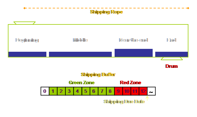
drum-buffer-rope was initially described with a two-zone buffer; comprising a
green zone and a red zone. However the
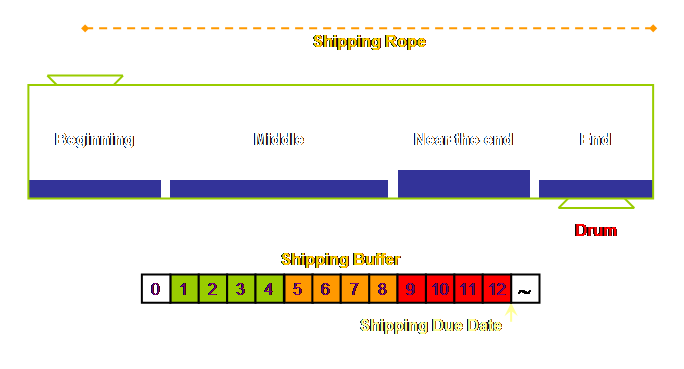
authors, being pragmatists, have since revised this to the basic 3 zone
buffer as we have used throughout here.
So, let’s redraw the system with a 3 zone buffer.
Simplified drum-buffer-rope, although developed as a
consequence of make-to-order systems moving towards the desired position of
being market constrained, is an ideal system for operating a make-to-stock
operation. In the following sections
we will look at, firstly, a transitional system that uses full “traditional”
drum-buffer-rope for make-to-stock and then, secondly, develop the argument
for using simplified drum-buffer-rope – first in make-to-stock and then in
make-to-replenish. Right now, however,
we must introduce the concept of stock buffers. There are two places where the supply chain
interacts with manufacturing – at the beginning of the process and at completion. It isn’t much good to have excellent
on-time service for make-to-order if we don’t have the necessary raw
materials on hand to begin with, nor is it very useful in make-to-stock if we
don’t have sufficient resultant stock-on-hand at all times. Often we don’t even think of raw materials
(or inwards goods) and finished goods as a part of the supply chain, they
seem, and in fact they are, integral to the manufacturing process. But by their very nature they are the end
of one supply chain, and the beginning of another. In supply chain each and every node for each and
every stock becomes its own buffer.
Each node must contain sufficient stock to meet demand (and variation
in demand) during the period from the beginning of one re-order/resupply
cycle to the next. In both
make-to-order and make-to-stock environments a stock buffer for raw material
input occurs at the beginning of the process.
In manufacturing make-to-stock environments a stock buffer for
finished goods output also occurs at completion. Let’s add these stock buffers to our
diagram.
To understand why we buffer these stock positions
just prior to, and just after, manufacturing in units of material rather than
units of time we need to consider how we determine both the stock buffer
activity and the stock buffer size. Let’s examine stock buffer activity first. Why do we use units of material for stock buffer
activity when we use units of time for the constraint, control points, and
shipping buffer activity? The reason
is that now the number of units is invariable but the amount of time or
demand that they “cover” is variable.
Sometimes demand is high and we utilize the same number of units
faster and over a shorter period.
Sometimes demand is low and we utilize the same number of units more
slowly and over a longer period. But a
unit is still a unit. Thus; At a stock node a unit is a unit but the
hours may differ The selection of units of time or units of material
isn’t arbitrary; it is based on the nature of the step we wish to
protect. If time is invariant (an hour
is an hour) then we use time. If
quantity is invariant (a unit is a unit) then we use quantity. Maybe it is much simpler to say that; We protect stock with a stock buffer What about the stock buffer size then? The unique perspective brought about by the
designation of a stock node allows us to define the length of the stock
buffer in time. Essentially the buffer
is sized and “sees” a duration that extends through one period of the
re-order/resupply cycle. However, the
buffer now “sees” uncommitted demand – we can not tell how much we
will sell in the next hour or the next day or whenever. Therefore, we must once again substitute
“non-variable” units of stock in place of the variable amount of time or
demand that they “cover.” Thus the
replenishment buffer size is also measured in units of quantity. We will return to the part the
re-order/resupply time plays in determining the stock buffer size soon. In many make-to-stock systems it might be inelegant
but never-the-less quite effective to give make-to-stock orders a due date
for completion as we would in make-to-order jobs and to therefore operate a
shipping buffer. The shipping buffer
then supplies a stock buffer. The
stock buffer itself will also contain some measure of safety. This undoubtedly overdoes the safety
aspect, as we have system safety in safety stocks and we have system safety
in the shipping buffer. However, so
long as this is recognized, and so long as it works, then it shouldn’t be a
problem. Let’s have a look at such a re-order system using full drum-buffer-rope.
In traditional reorder approaches to make-to-stock
using min/max systems we can “wing” a reorder system using recent rates of
consumption to give us a “time remaining until order release.” Orders with the least time remaining get
priority. Priority = [(Stock-On-Hand + Work-In-Process –
Orders) – Reorder Point] / Consumption Such an arrangement of course also allows for a very
effective mixed make-to-order/make-to-stock operation. Probably the greatest majority of
businesses currently operate in this manner.
This transitional example is shown with an internal
constraint. In this case we can try
and supply all of the demand but it is not possible. Therefore, either we must accept that some
of the stock buffers will be out-of-stock some of the time, or we must reduce
the total number of stock items – just as we must turn down some orders in an
internally constrained make-to-order system.
Despite the protests of purists, make-to-stock systems often start
from this position but it isn’t so easy to recognize. In an internally constrained make-to-order system
the turning down of orders is often active; we make a decision to do
so. In an internally constrained
make-to-stock system the decision is sometimes passive; the customer
makes it for us. Moreover the customer
may never “voice” disappointment at a stock-out, they may simply go elsewhere
and we might not ever know. Really, we want our initial internally constrained
make-to-stock operation to move towards being market constrained. Think about it. We need sufficient stock so that our customers
can always find what the want, and when they want. Such market constrained systems tend to be
replenishment systems which we will discuss in a moment. The objective of this transitional and
traditional drum-buffer-rope stage is to make available the needed capacity
to get to the required level of output.
The identification, exploitation, and subordination steps of full
drum-buffer-rope will uncover existing capacity that was previously
unrecognized. We need to understand why this transitional stage is
so common. One reason without doubt is
that materials requirements planning (mrp) and material resource planning
(MRP II) use time as the default for treating stock orders. This is so common that we don’t even
challenge the assumptions behind it.
To do so however, we need to introduce a new concept. We need to introduce the concept of replenishment
stock buffers. As we move from being internally process
constrained, to being externally market constrained – a normal consequence of
implementing drum-buffer-rope – then there is an opportunity to move from
fixed-quantity variable-frequency make-to-stock to something superior. We will call this superior mode of
operation make-to-replenish – as distinct from make-to-stock. First, however, we need to be aware of a
subtlety. We need to remind ourselves
of our plan of attack, our 5 focusing steps.
They are; (1) Identify the system’s constraints. (2) Decide how to Exploit the system’s constraints. (3) Subordinate everything else
to the above decisions. (4) Elevate the system’s constraints. (5) If in the previous steps a constraint has been broken Go back to step 1, but do not allow inertia to cause a
system constraint. In other words; Don’t
Stop. We know that the constraint is in the market, so
where then is our leverage point?
Using the terminology of Dettmer (13) it has to be somewhere within
our span of control rather than our sphere of influence. Just as the due date was a seductive place
to consider leveraging from in make-to-order, so too here is the finished
goods stock. After all, we must have
the right material in the right place at the right time –
always. However, just as with due dates in make-to-order,
the greater the difference between the additional capacity of the internal
weakest link and the market demand; that is the amount that internal capacity
exceeds external demand, the smaller the queue in front of the weakest link
and the shorter the manufacturing lead time and thus the smaller the stock
buffer that is required. Conversely,
the lesser the difference the greater the queue in front of the weakest link,
the longer the manufacturing lead time, and thus the greater the stock buffer
that is required. Again, it is the
characteristic of the timeliness of the system that is important and it is
the interaction of the internal weakest link with the overall system that
determines this characteristic. It is
from the internal weakest link that we leverage the whole system. Does that seem logical? Then let’s move on. In a make-to-replenish environment, stock provides
the system safety against both the variation in demand from the customer and
variation in the time to needed to re-order and resupply the stock. Therefore we don’t need to use a shipping
buffer; the stock is our buffer. This is an ideal system, let’s see how it looks,
let’s draw this new system.
Replenishment buffers characteristically oscillate
between being nearly full and being somewhat empty. They oscillate between zone 3 and zone 2 –
rarely do they move into zone 1.
Movement into zone 1 is a signal for management action (action by
exception). If having 1/3rd of your
stock “sitting” in zone 1 sounds wasteful remember that this system is
frequency driven. Total finished goods
stock may well be 1/2 or 1/4 or even less of that previously required at this
first stage after manufacturing. Let’s
check that we understand why. In the earlier discussion on drum-buffer-rope
make-to-order we limited ourselves to the benefits that occur when excess
work-in-process is removed from the system, we “dried the system out” by at
least 50%; and lead time was reduced proportionally. We didn’t consider the “what if” when an
order consists of 1000 units of the same thing, surely we could manufacture
that as two lots of 500? In a way we
would have been getting ahead of ourselves, in fact the whole subject of
batching is so important that there is a further page on it called “batch
issues.” However, because batching is
endemic to make-to-stock we need to address it here to some extent. So let’s ask the what if. What if we have a batch of stock of 1000
units, and what if we made two smaller batches of 500 units instead? Well, each batch would move through the
process twice as fast as before. The
rationale is that most of the time that a batch spends on the floor is time
spent waiting, and therefore a batch of 500 waits half as long as a batch of
1000. Unconvinced about the
waiting? Go attach a balloon to a
batch or two and see what they are doing over a couple of days. So, if we dry the system out of excess
work-in-process and that reduces lead time by at least half, and then we
reduce batch size in-turn by half that will reduce lead time to a quarter –
without even trying. Of course we have
to run those batches twice as often, could that be a problem? Well not usually. It is not a problem as long as we don’t
turn a non-constraint into a constraint by too many set-ups. Now let’s look at two further considerations. Firstly; we don’t batch when we
replenish! Oops. Trying not to use the term “batch” from now
on is going to be so darn difficult, however, it is not politically correct
to talk about fixed-batches in replenishment
because they don’t exist, therefore we will talk about the variable replenishment aggregate size instead. As Schragenheim points out, in all of the
standard approaches to make-to-stock there is a buried assumption somewhere
as to a fixed batch size (8). We
assumed exactly that in our transitional approach above. So yes, common sense tells us that we must
aggregate some of the stock units some of the time, least we grind the system
to a halt, or we are Toyota, or we are very clever. However, we should strive to keep the size
of our replenishment aggregate as small as possible and variable; that
is, not invariably the same size each and every time. Secondly; we may have product
cycles. Sometimes when the
nature of the material is different for different stock we may wish to make
everything required with one material before we change to another. Or we might have a preferred sequence of
set-ups either up or down the size range or some other set of dependencies
that cause us to cycle through our manufacturing process. The good news is that cycle times will
decrease in proportion to our variable replenishment size reduction. Why is this so important? It is important because our
initial stock buffer size, and hence the physical inventory and financial
investment that we must carry, depends upon the resupply time. In the absence of product cycles and large variable
replenishment aggregates the manufacturing lead time determines the
resupply time. In the presence of product cycles, the time
for the completion of a cycle plus the manufacturing lead time
determines the resupply time. There is a more detailed explanation of the
characteristics of replenishment in the second part of the replenishment page
in the supply chain section. Be aware
that manufacturing professionals tend to misunderstand replenishment at first unless they have been
exposed to supply chain management. If
we have only ever been exposed to fixed batches of material then everything
tends to look like a fixed batch of material.
This is a very real and substantial block. Please check the replenishment page to test
your understanding. During the implementation phase of simplified
drum-buffer-rope in a make-to-replenish environment the removal of fixed
batch sizes and replacement with smaller more frequent variable
replenishment size orders is the critical parameter in determining system
behavior. If the demand in make-to-replenish is uncommitted,
then how do we plan? Well, the same
way as in make-to-order simplified drum-buffer-rope, we load replenishment
orders against our aggregate capacity – our daily or weekly capacity
multiplied by the material release rope length. The capacity is defined as that of the
weakest link in the process. We
shouldn’t fill more than about 80% of that capacity over any medium term
plan. Let’s add this to our model.
The amount of stock that we must hold in our stock
buffer depends upon the amount of time that it must “cover” for. The principle components of that time are
the reorder time and the resupply time.
We can define the stock buffer as follows; Finished Goods Stock Buffer = Average Demand x
(Average Re-order & Re-supply Time) Because we use averages for demand and for time we
use the margin of safety to accommodate that which we know least well, the
variation around the average values.
If the resulting buffer is too big it will soon become apparent and we
can, in fact we must, resize it.
Likewise, if the buffer proves to be too small then we will also have
to resize it. Re-order and resupply time are clearly the most
critical components. We have already
discussed the factors that lead to a reduction in resupply time, most of
which are within our own control; what then are the issues that determine the
re-order frequency? Policy of course! Whose policy? Our policy! Yep, there are not a whole lot of excuses why
re-order, which is totally under our own control in our own system, can not
be substantially reduced in duration.
If we are big enough to have a real problem then we will have a
computer and that can easily be interrogated more frequently. If we are small enough to have no problem
then we just need to do the sums more frequently. In drum-buffer-rope make-to-replenish, buffer
management once again provides us with both local control via buffer status
and global feedback in the form of buffer resizing via longer term trends in
buffer behavior. The model is the
same; the terminology is modified to suit the environment.
Stock buffer status is defined in the same way as a
time buffer; Stock Buffer Status = (Buffer Quantity –
Stock-On-Hand) / Buffer Quantity We have already used this concept with buffers for
work orders in make-to-order, exactly the same principles apply for stock
buffers in make-to-replenish. Let’s
illustrate the concept with a few diagrams for stock buffers. The following buffers contain varying
amounts of stock-on-hand (SOH).
Of the other buffers; C is in the green zone, zone
1, and of no concern, buffers A and D are within the yellow/orange zone, zone
2, and we should leave well alone unless we once again wish to tamper with
the system – and Deming taught us what happens when we allow that occur. So let’s not do it. By using buffer status we can prioritize different
product buffers amongst each other regardless of whether one replenishment
buffer covers a period of 2 months and 2000 units and another replenishment
buffer covers just 2 days and 20 units. In make-to-order the relative priority of released
work orders can only be affected by internal “things,” however, in
make-to-replenish the relative priority of stock orders can also be affected
by external changes in the market demand during the processing time. Because stock orders should be smaller and
more frequent it is also possible that more than one order for identical
stock can be in-process at the same time, this too must be taken into
consideration. Thus the stock order status for material on the
floor is (8); Stock Order Status = (Buffer Quantity –
Stock-On-Hand – WIP Ahead) / Buffer Quantity Let’s illustrate this with two different stock items
– “light blue” and “lavender.”
Buffer status tells us about the end condition of
the system and whether to check or maybe facilitate work already released for
production. However, without customer
due dates as in make-to-order jobs, how can we prioritize new jobs for
material release? To do this we must
replenish the buffer to its full capacity allowing for current stock-on-hand
and current work-in-process, thus; Stock Release Priority = (Buffer Quantity –
Stock-On-Hand – Total WIP) / Buffer Quantity For the example that we just used with “lavender”
and “light blue” finished goods stock buffers, we have the following release
priorities.
The actual amount of material released to replenish
the buffer will be the amount required to bring it be back to the full buffer
quantity; Stock Replenishment Quantity = Buffer Quantity –
Stock-On-Hand – Work-In-Process When demand is generally high, then the time between
one stock order being released and the next order for the same stock will
increase because each order is now larger and takes longer to process,
however overall system set-up will decrease as a consequence. Conversely, when demand is light, the time
between each order will decrease because each order is now smaller and takes
shorter time to process. Overall
system set-up will increase as a consequence.
Schragenheim argues persuasively how this mechanism self-adjusts to load
and can be used to drive system stability (8). Do you notice something important? We have moved away from fixed batch sizes and away from the fixed schedules of transitional
make-to-stock. The re-order frequency
and resupply frequency and quantity are now totally determined by the
characteristics of the system that we implement and the demand
characteristics of the customers. This
is make-to-replenish. In fact we are not entirely free of fixed
schedules. In replenishment we have at
the very least; rechecking, re-ordering and resupply. The re-ordering and resupply are indeed
free from fixed-frequency scheduling but there is one last hold-out – the
rechecking. Most likely we will still
batch this in time – to once a day, towards the end of the day maybe when we
“know” what we have sold that day. There is an alternative stock buffer sizing rule for
finished goods stock buffers.
Schragenheim and Dettmer use the term “emergency level” to define zone
1; they suggest that zone 1, the red zone or emergency level, should contain
sufficient stock to cover the time required to expedite a medium size
replenishment order through the system (14).
Three times this value will therefore define the full buffer size. Let’s make sure that we understand all of the terms
that apply to a stock buffer, let’s use the light blue buffer as an example.
A make-to-order system has just one, or maybe two,
buffers – either the shipping buffer or a constraint buffer and a shipping
buffer. In essence the system must
always have a drum buffer.
Make-to-stock therefore seems overwhelming because every stock buffer
becomes a drum. Thus we have move from
just one or two buffers to maybe many hundreds or even thousands of
buffers. Nevertheless we need to
address both the aggregate behavior of the buffers and their individual
behaviors. A buffer hole occurs whenever there is an incursion
into zone 1, the red zone, of the buffer.
Let’s draw this for a stock buffer.
Unlike make-to-order where each job is discrete and
a buffer hole can be quantified when the job is finally completed,
make-to-stock is continuous – we continuously replenish and customers
continuously deplete our replenishment.
So we can not put a mark in the ground that says “hole closed on this
day.” Instead we must continuously
monitor the number of units missing and the number of days that they are
missing from zone 1. This is the
measure that will tell us what is happening in individual buffers. We must record the number of units “missing” from
zone 1 each day that any units are missing and we must aggregate this over
our reporting period – be that a day, a week, or a month. The measure is unit-days late. From the buffer hole data we can construct a more
meaningful measure. One that includes
the value of the problem. In a
for-profit environment these are known as throughput-dollar-days (late) and
inventory-dollar-days (wait). Let’s
add these to our diagram.
Throughput-dollar-days late is our unit-days of material
missing from zone 1 of the buffer multiplied by the expected throughput of
the product. This way both the size of
the hole and the value placed in jeopardy are taken into account. We must remember that the purpose of a
buffer hole is an internal warning to us that we may “ping” a customer. Throughput-dollar-days tells us how loud
that ping could be – of course we will absolutely strive to remedy the
problem before it reaches the customer. Inventory-dollar-days has an important role in
make-to-replenish. No-longer does it
just protect us from gaming the system – having no zone 1 penetrations by
loading excess work-in-process; it now alerts us to the ageing of stock. What if the risk of “pinging” a customer becomes
more frequent and greater? Surely this
must be a message that we need to increase the size of the particular buffer
concerned – unless of course we want to spend all our time and energy
fire-fighting (and we put our fire-fighting gear away – right?). So buffer penetrations that are too
frequent into zone 1, the red zone, require an increased in buffer size. Conversely, buffers that are always in zone 3, the
green zone, indicate a need for reducing the size of the buffer. We monitor the behavior of our protection and if it
is insufficient, or if it is over-protective, we make adjustments to the
system to accommodate this. In the earlier re-order system we were able to mix
make-to-order and make-to-stock by giving make-to-stock orders a due
date. In mixed
make-to-order/make-to-replenish we can do away with the due date for
stock. Essentially we have two
drums. We have two drums because we
have two markets; those that can’t wait (make-to-replenish) and those that
can or must wait (make-to-order). The
typical situation here might be standard items (make-to-replenish) and
special one-off items (make-to-order) – even though we might make several
hundred or several thousand units in one male-to-order. Of course the aggregate load of the two
drums can’t exceed the availably capacity of the most capacity constrained
internal resource. But then simplified
drum-buffer-rope allows us to load against that aggregate capacity. How does this look, let’s see.
We would hate to sacrifice a late make-to-order job
because we thought the demand for a make-to-replenish order was more urgent,
only to then find out that the make-to-replenish wasn’t urgent at all – the
demand had dropped away again. How can we
manage such a duality? We are dealing
with both time (make-to-order) and with quantity (make-to-replenish). Well, Schragenheim shows us how; with the
buffers of course. Let’s have a look.
This is the power of Schragenheim’s buffer status
methodology. “Even though the
calculation of the buffer status is different, they are fully comparable
(8).” It seems almost quaint now, but in 1986 when
Goldratt and Fox wrote The Race, the
role of reduced inventory was still, in many peoples’ minds, an open
question. Never-the-less, they
proposed six competitive edge issues built around; product, price, and
responsiveness, in which reduced inventory has a positive effect and set out
to demonstrate their case (15). These
issues are listed below.
Their demonstration of the case is the reason for
accepting in the measurements section that inventory reduction does in fact
have a positive impact via future throughput on the bottom line measure of
net profit. Of course time also
appears to have substantiated the importance of inventory reduction in all
six cases. The objective of Theory of Constraints and
drum-buffer-rope however is not to reduce inventory per se,
it is to increase throughput – the rate at which the system produces money or
goods or services in order to move the system towards its goal. Most often inventory reduction is a
desirable and feasible outcome; but it supports the objective of increased
throughput, it is not an objective itself. Making Throughput the objective in Theory of Constraints
is quite different from other approaches.
In the pursuit of bottom line improvements traditional cost management
focuses primarily on reducing operating expense, and is neutral about
inventory. Just-in-time focuses
primarily on reducing inventory, and is neutral about operating expense. Constraint management focuses primarily on
increasing throughput and is neutral about operating expense. We can illustrate this as follows;
All three approaches; traditional management,
just-in-time, and constraints management are naturally interested in
increasing throughput, but only constraint management has this as its primary
focus. Let’s run past this in a different direction. Just-in-time, and to some extent kaizen,
are noted for actively lowering inventory in search of problems. The exposed problems are then resolved and
throughput may go up as a consequence.
Theory of Constraints is almost the reverse. It is noted for actively seeking out
problems to increasing throughput. The
problems are resolved and inventory may go down as a consequence. Problem solving via inventory reduction is well and
good for work-in-process, but what about raw material and inwards good
then? Reducing raw material inventory
only to find the problem is with a vendor is not especially useful unless the
vendor is willing to improve. Don’t
let just-in-time zealousness erode protective raw material supply. Just-in-time works in Japan because the
obligations of mutual interdependence are much greater. In Western businesses, if there is a
particularly unreliable vendor then, at the very least, we must protect
ourselves with as frequent as possible small-lot replenishment. Let’s explore this further. Many businesses, especially make-to-stock, have
standard common raw material or inwards goods items that are keep as
stock-on-hand. Essentially theses are
raw material stock buffers. In the
introduction to raw material and finished goods buffers we remarked that raw
material is a more exacting environment than finished goods. Why is this? Well, ask any purchasing officer or
in-wards goods officer who failed to have the right material in the right
place at the right time for production.
In reality we have almost no control or authority over the external
re-supply chain and yet we are expected to assume full responsibility for
managing the goods within it. How do
we best protect our system in this case? Let’s draw our simple raw material stock buffer
feeding our production system and work outwards from there.
Inwards Goods Stock Buffer = Maximum Demand x
(Average Re-Order & Re-Supply Time) The key point is that we must accommodate the
maximum anticipated demand and the maximum unreliability of the vendor. We are really applying Goldratt’s first two
rules of business; (1) “be paranoid,” and (2) “be paranoid.” The 3rd rule is also useful – “don’t get
hysterical.” We guard against hysteria
by frequent re-orders. Why? Let’s see. The replenishment time is composed of up to 4 components; (1) Our re-order frequency – and hence
duration (2) Vendor cycle frequency – and hence
duration if it is not ex-stock (3) Vendor process lead time – and
hence duration if it is not ex-stock (4) Vendor order processing &
shipping frequency – and hence duration We have control over just one of those issues, our
own re-order frequency. We should make
sure that this is not a policy problem of our own making. With these exceptions, we can otherwise treat raw
material or inwards goods stock buffers in the same manner as we have
discussed for finished goods stock buffers. If this explanation of drum-buffer-rope,
make-to-order, make-to-stock, and make-to-replenish seems quite simple and
straightforward then that it excellent; we have an understanding of the
underlying fundamentals. If experience
tells us that reality is more complicated than these simple I-plant examples,
then that too is excellent. Now we are
in a position to better understand how to apply this methodology to more
complicated V-plants and A-plants. The best place to begin to get a better idea of how
to apply drum-buffer-rope to a particular situation is a set of diagrams for
more complex layouts in The Race
(16). The
Constraints Management Handbook also deals with V-A-T issues at
length (17). The whole second volume
of Synchronous Management is devoted to
implementation issues in V, A, and T-plants (18). The production simulator in Production the TOC Way (19) allows us to run
computer-based simulations of whichever type of plant is relevant and to
learn “first-hand” what we need to do in order to move towards our companies’
goal. The simulator is a tested and
true approach – try it. You will gain
more in two days using a properly facilitated simulator than two months of
other endeavors. There is also a more recent subset of the production
simulator with a slightly different interface made available as the TOC Executive Challenge (20). This is another excellent way to develop
understanding in a “safe” (read virtual) environment. Stein’s book Re-engineering The
Manufacturing System (21) details the algorithms for the “Haystack
Compatible” scheduling system that is the more complete expression of the drum-buffer-rope
make-to-order core described here. Of
course Goldratt’s book The Haystack Syndrome does
this as well but in a more concise way. Finally, incorporated within Warp Speed
(22), Schragenheim has made available a “Management Interactive Case Study
Simulator” or “MICSS” for short. This
offers a rather sophisticated ERP view on a simple linear plant with the
opportunity to run the plant under a number of different logistical systems
(MRP, DBR, S-DBR) and to evaluate the effect of different policy changes on
the outcomes. It is a very effective
tool for self-study and group-learning. The revised edition of the TOC production simulator
and the “Insights” introductory material make some subtle changes to how we
define some buffers. The older set of
definitions has been used on this web page, however, a concise discussion and
comparison of the two sets can be found on a short sub-page here.
Here we presented drum-buffer-rope within the
context of the 5 focusing steps, our plan of attack. The fourth step reminds us to then
strengthen the weakest link and the fifth step contains an important
admonishment – don’t allow inertia to become a system’s constraint. In other words drum-buffer-rope isn’t just
a method of identifying and protecting the weakest link, it is a process of
robust, continuous, and on-going improvement. Understanding the generic solution is well and fine,
but now we also do need to look at some of the necessary detail of actual
implementation. Let’s do that next.
(2) Goldratt,
E. M., (1990) The
haystack syndrome: sifting information out of the data ocean. North River Press, pg 146. (3) Goldratt,
E. M., (1997) Critical chain. The
North River Press, pg 149. (4) Stein, R.
E., (1996) Re-engineering the manufacturing system: applying the theory of
constraints (TOC). Marcel Dekker, pg
143. (5) Goldratt,
E. M., (1990) The
haystack syndrome: sifting information out of the data ocean. North River Press, pg 128. (6) Schragenheim,
E., and Dettmer, H. W., (2000) Manufacturing at warp speed: optimizing supply
chain financial performance. The St.
Lucie Press, pp 123-135. (7) Schragenheim,
E., and Dettmer, H. W., (2000) Manufacturing at warp speed: optimizing supply
chain financial performance. The St.
Lucie Press, pg 176. (8)
Schragenheim, E., (2002) Make-to-stock under drum-buffer-rope and buffer
management methodology. APICS
International Conference Proceedings, Session I-09, 5 pp. (9) Goldratt, E.
M., (1990) The
haystack syndrome: sifting information out of the data ocean. North River Press, pp 206, 209, 241. (10) Caspari,
J. A., and Caspari, P., (2004) Management Dynamics: merging constraints
accounting to drive improvement. John
Wiley & Sons Inc., pg 180. (11) Goldratt,
E. M., (1990) The
haystack syndrome: sifting information out of the data ocean. North River Press, pg 136. (12)
Schragenheim, E., and Dettmer, H. W., (2000) Manufacturing at warp speed:
optimizing supply chain financial performance. The St. Lucie Press, 342 pp. (13) Dettmer,
H. W., (1997) Goldratt’s Theory of Constraints: a systems approach to
continuous improvement. ASQC Quality
Press, pg 67. (14)
Schragenheim, E., and Dettmer, H. W., (2000) Manufacturing at warp speed:
optimizing supply chain financial performance. The St. Lucie Press, pg 177. (15) Goldratt, E. M., and Fox, R. E., (1986) The
Race. North River Press, pp 36-67. (16) Goldratt, E. M., and Fox, R. E., (1986) The
Race. North River Press, pp 96-105. (17) Cox,
J. F., and Spencer, M. S., (1997) The constraints management handbook. St Lucie Press, pp 101-128. (18) Umble, M. M., and Srikanth, M L.,
(1997) Synchronous management: profit-based manufacturing for the 21st
Century. Volume 2 implementation
issues and case studies. The Spectrum
Publishing Company, 234 pp. (19) Goldratt, E. M., (2003) Production
the TOC way (revised edition). North
River Press. (20) Tripp, J., (2005) TOC Executive Challenge: a
goal game. The North River Press
Publishing Corporation, 56 pp. (21) Stein,
R. E., (1996) Re-engineering the manufacturing system: applying the theory of
constraints (TOC). Marcel Dekker, pg
190. (22)
Schragenheim, E., and Dettmer, H. W., (2000) Manufacturing at warp speed:
optimizing supply chain financial performance. The St. Lucie Press, 342 pp. This Webpage Copyright © 2003-2009 by Dr K. J.
Youngman |