|
A Guide to Implementing the Theory of
Constraints (TOC) |
|||||
|
How Do
We Implement Drum Buffer Rope? In the
previous section we examined the mechanics of drum-buffer-rope in a rather
basic form – an idealized framework. In this section let’s try to flesh out this
framework with a little more implementation detail. Of course the best way to learn this detail
is to just to go out and do it.
Drum-buffer-rope and the Theory of Constraints is a robust methodology
so long as we keep the rules of engagement and plan of action in mind. We will use
the 5 focusing steps – our plan of attack – as our template. We probably can’t repeat these steps too
many times so let’s repeat them again right here; (1) Identify the system’s constraints. (2) Decide how to Exploit the system’s constraints. (3) Subordinate everything else
to the above decisions. (4) Elevate the system’s constraints. (5) If in the previous steps a constraint has been broken Go back to step 1, but do not allow inertia to cause a system
constraint. In other words; Don’t
Stop. OK then, let’s
start at the start. In any normal
production process, either manufacturing or service based, there will be
work-in-process everywhere, especially if the plant is run as a balanced
line. Even more so if you use some
form of MRP or ERP. How do we find the
weakest link? In this situation every
step looks like the weakest link with large amounts of working waiting to be
done at each stage. There are 3
ways; (1) Find the step with the longest waiting time for work to be completed. (2) Find the step that most often causes disruption downstream. (3) Nominate something. Doing
something, anything, might seem counterintuitive, but if you haven't chosen
the real constraint, then it will make its presence felt very quickly. This
is a process of on-going improvement; don't be scared to do something –
anything – because each step will take you closer to your company's goal. No, no. Please don’t do this. Collecting data and writing a report should
not be considered as doing something, at least not something that effective
people do. Most likely it should be
considered as doing nothing. Data
collection is usually a stalling tactic.
The data is never good enough to make a decision on – which means you
will need to collect even more data.
Remember this is a dynamic complexity problem, so don’t go and use
detail complexity solutions such as searching for more accurate data on
it. Normally with drum-buffer-rope you
should have demonstrable results in the same amount of time as others would
have spent collecting data. So it
becomes a choice, take an action, or collect data. Moreover,
report writing usually doesn’t generate ownership or understanding of the
real problem, it might generate an understanding of the symptoms, but not
usually of the underlying core problem or core conflict. Reports generally do not involve all the
needed people and are usually perceived to apportion blame. Note, perceived to apportion
blame. So even the most neutral and
factual report will be perceived by some people – usually the people in the
problem area, to be apportioning blame.
There is usually only one response to this by the people involved,
defensiveness and deflection of the perceived blame onto another area. Naturally enough this will not help to
improve things at all. The Thinking
Process graphical trees are the tool of choice for generating buy-in and
understanding of the problem and then seeking consensus on the solution. In addition
don’t be afraid to go and stand in the middle of your process and just watch
what is happening. People will get
used to you being there fast enough.
And you are in good company, Taiichi Ohno the inventor of Toyota’s
just-in-time once said; “We can talk about work improvement, but unless we
know production thoroughly we can accomplish nothing. Stand on the production floor all day and
watch – you will eventually discover what has to be done. I cannot emphasize this too much (1).” It is likely
that people with an affinity for understanding flow will naturally spend
considerable time on the floor; don’t be afraid to do this just because no
one in the company has done it before.
This is the reality check between what people tell you is happening in
production and what really is happening.
The Japanese have a saying; go to the actual place, see the actual
problem, and speak to the actual people.
Just common sense really. Almost all
implementations in the pre-drum-buffer-rope stage claim to have wandering
bottlenecks. Don’t worry, there will
almost certainly be work-in-process everywhere as well, and this is the cause
of the impression. However, later – as
things begin to flow – there may still be the impression that there are
wandering bottlenecks from time to time.
In this instance it is most likely a case of wandering large
batches. Large batches will hold
themselves up at slow process stages.
Reduce the maximum batch size and the problem will go away. Usually the
people in the process have the best idea of where the constraint might
be. If all else fails then just
nominate something, and the real constraint will make itself known within a
short space of time. Initially the
constraint is protected by a large pile of work-in-process; there is always
something to do. But is the constraint
always doing something productive? Is
the constraint sometimes doing things that are unproductive? The best way to find this out is to write a
plan, a schedule for the constraint.
If you already have schedules for the plant in place, this might be
the very first time that you write a schedule in detail for one
resource. This can be as simple as a
whiteboard on the production floor.
The important thing is to write a plan of how to exploit the
constraint over the next short period.
Then we have a basis to evaluate our actions and our results. The schedule will let you peel away the
obstacles to proper exploitation one by one. Exploitation
tactics on the constraint in manufacturing include; making sure automated
machines run during breaks, making sure set-ups are staggered, fixing
break-downs quickly (or preventing them completely), replacing absent workers
quickly, avoiding downtime during shift changes, avoiding multitasking of
set-up personnel, keeping faulty work or unnecessary work off the constraint. Of course
people will have always tried to do this; it is just that they didn't know
where to focus on in the past. Now
they do. The focusing itself will
greatly improve the constraint. For
example when management sees the set-up man on the constraint waiting for a
laptop to program a machine and that the laptop is currently at some
non-constraint machine on the other side of the plant, they will take
action. Whereas one week prior the
only action would have been to ask the constraint operator to be patient. This doesn’t
have to be sophisticated – especially if your operation isn’t particularly
complex. Even if your operation
appears complex prior to drum-buffer-rope, you might be surprised how it
looks with in a few short weeks. A
constraint schedule might be written on a white board on the work shop floor,
or a sheet of graph paper, or travelers/paperwork hung in sequence on a rope
near the constraint. The
synchronization might not be anything more than one job finished at the constraint
means one job admitted by the gating operation. The important thing is that is understood
and that it works. More complex
operations in all likelihood already have an infinite capacity MRP-based
scheduling system in place and then it is a matter of adjusting this to work
in a finite capacity drum-buffer-rope environment. There are drum-buffer-rope schedulers
available, for instance see Manusync in the links and resources, however it
is infinitely better to get the organizational understanding and behavioral change accomplished first and then
look at more automated options and to leverage off the automation. Automation before understanding is like
putting the cart before the horse and it is not known to be effective. What if, for
some reason, the actual constraint is difficult to schedule? No matter, you could consider nominating a
shadow constraint somewhere else – just make sure that it is “hobbled” by the
schedule so that it can’t exceed the throughput of the real constraint (2). When the schedule
and reality deviate for whatever reason, then schedule reality. Generally this means re-synchronizing the
current constraint sequence to a new time.
Of course proper buffer management should avoid such resynchronization
– but stuff happens.
We must ensure
that we subordinate our local actions to that of the goal (global outcome) of
the system. For actions read;
decisions, behaviors, measurements, and policies. Normally we do that via the plan we write
for exploiting the constraints – the schedule. When we have a
written exploitation plan in place we can quickly compare actual results
obtained with the planned results. We
will soon see deviations. As we saw in
the section on process of change, these deviations from the plan results from (12); (1) Not
doing what was supposed to
be done. (2) Doing what was not
supposed to be done. The deviations
from plan result from our failure to properly subordinate. Let’s have look at some the more common
subordination issues in more detail. Then we will look at two local performance
measurements that we can use to align and monitor our subordination efforts
with. We will also consider a pivotal
role in subordination; the role of the buffer manager.
It is not
enough to write a schedule, we must also protect the constraint to make sure
the correct material is always ready and waiting for processing in good time
before the start date at the constraint.
We can achieve this by ensuring that we release material a rope-length
in time prior to the scheduled consumption on the constraint. Previously we
applied a rule of thumb which was to make the rope length half the current
lead time from gating release to the constraint start time. We then divided this rope length into 3 equal
buffer zones. Essentially we expect
most jobs to be ready and waiting at the buffer origin (a place in front of
the constraint) within 2/3rds of the buffer time available. But just how much is most? It seems to vary; original estimates seemed
to be of the order of 90% (4). More
recent estimates suggest 95% (5). It
seems much more likely that the actual percentage is best determined by the
volume of jobs in each situation. Even
though zone 1 was called the expediting zone initially, more recent terminology
seems to favor dropping this term and simply calling it zone 1. Expediting has such negative connotations
in manufacturing. There is some confusion however in the literature
over the definition of the buffer. In
fact this confusion arises more as a consequence of the difference in
interpretation between the buffer and zone 1 of the buffer. The total buffer time is divided into 3
parts. The zone closest to the buffer
origin should normally “be full.” Some
authors then call this zone 1 component of the entire buffer as “the buffer.” Schragenheim and Dettmer, Stein, Caspari and Caspari
follow Goldratt’s lead and take a total lead time approach to the buffer
definition (6-8). Woeppel, Cox and
Spencer, and Umble and Srikanth take a zone 1 definition of a buffer (9-11),
that is they treat it as a discrete addition of time in front of the
constraint. It seems that those who
relate more closely to MRP environments prefer the zone 1 definition of a
buffer. Sometimes a zone 1 definition of the buffer helps
people to understand the local versus global safety argument. Let’s have a look at that next. Umble and
Srikanth were perhaps the earliest to publish on the detail of
drum-buffer-rope independent of Goldratt.
They chose a Zone 1 definition of the buffer (11). Basically this develops out of an argument
for local safety everywhere versus safety as strategic buffers in a few key
places. Probably few
managers would deny the importance of a special buffer in front of an
identified constraint – many more, however, would be hugely reluctant to give
up their local safety everywhere else.
They would prefer to keep all their local safety and create some
additional safety in front of the constraint. Because the
concept of local safety everywhere is second nature to manufacturers it is
sometimes difficult for managers to see the important characteristics of
global buffers. As previously
mentioned, if an MRP or ERP system has been implemented, the local safety
values might be quite explicit. If you are
interested the argument for moving from local safety everywhere to global
safety in a few key places is here. Proper
subordination not only means making sure that we use the right measures, but
also means making sure that the right measures are continuously communicated
to the line. The most important global
measure is physical output and/or financial throughput. If the constraint is internal then this
should go up, if the constraint is external then it may initially stay
constant, but it too should go up. These results should be visible to
everyone and updated as frequently as possible. Updating once a day is good and is not too frequent. But having visible results is not
enough. The line management must
reinforce positive results with a few well chosen words to the right people
at the right time. That reinforcement,
like water, will filter down to all levels and in all directions. Reluctance to
praise will be viewed as failure to support the initiatives. You would be amazed how some managers are
reluctant to praise significant results.
You can be almost sure that the manager concerned does not fully
support the implementation. It is a
very passive way of communication, do everything requested but say
nothing. Such managers can block
praise from the leadership meant for the line by failing to pass it on. It happens. By the same
token the leadership must reinforce positive results with a few well chosen
words to the right managers at the right time. Without that feed-back the managers may
decided that leadership support is lacking. All
implementations develop speed wobbles.
The analogy is a child who has just learnt to ride a bicycle, maybe
straight-off, or maybe for the first time without dummy wheels or stabilizers
or what ever you wish to call them. As
the child goes a little faster, at some stage they will decide that if they
go any faster they will fall off – and they do. Our people may never have produced as much
output before without some sort of assistance (overtime maybe), they
certainly won’t have done it with less inventory as well – they will convince
themselves that they can’t continue to do it and things will come unstuck for
a few days. And then we just pick
ourselves up again and go straight past the point where we thought we
couldn’t go past before. What is
really happening is that people are learning to subordinate properly for the
first time. We have
mentioned many times of the need to reframe the environment from one of a
reductionist/local optima approach to one of a systemic/global optimum
approach. One of the most important
aspects of this reframing in a processing setting is the perceived value of
work-in-process held by the guys on the floor. It is the epitome of local optima. A large pile of work-in-process in front of
each work center in the morning is a measure of importance and security to
the members of that work center.
Seeing that work-in-process moved to the next work center by the end
of the day is a measure of success and satisfaction to the members of the
work center who processed it. If we
reduce work-in-process in this setting then we must “unhook” these measures
of security, success, and satisfaction and “rehook” them to the global
measures of the system. People will
get used to the new reduced inventory way quite quickly, they will develop
pride in how “the work I started this morning is now way over there,” but it
needs careful nurturing and the positive reinforcement mentioned above during
the transition. If managers
find the importance of work-in-process hard to believe, then try operating
with a clean desk policy (a really clean desk) for a couple of days and count
the number of people who will question whether you have any work to do. These pressures are pervasive and very powerful and can undo an implementation. To properly
subordinate the process to the constraint we must pace new material release
to the pace of the constraint. To do
more only builds work-in-process. Many
times early on there are likely to be pressures to admit extra work. Often there are not-so-subtle pressures from
sales people to favor certain clients – always their clients and not anyone
else’s clients. It requires good
leadership in both sales and manufacturing to avoid this. Another reason for using the holistic
approach prior to the implementation. An important
part of subordination is to make sure that the “drumbeat” is relayed to the
start or gating operation and is observed. This means that new scheduled work should
not be admitted into the system any sooner than scheduled. Again in the early stages there is a great
temptation to admit work early to keep the next several stages “busy” and to
“get ahead” at little. Doing this will
result in non-constraints at some stage working on work that is not needed to
be worked on and not working on work that is needed to be worked on. Local work-in-process will go up, local
lead times may increase, and if this is a consistent policy, holes in the
buffer will surely arise, and throughput will go down. The
subordination challenge for gating operations and all other non-constraints
is to keep work-in-process and lead time low and constant and the buffer full
(downstream). To do this we must
protect their sprint capacity. The capacity
that all non-constraints have above and beyond the capacity of the
constraints is often termed protective capacity and sometimes called sprint
capacity (13). Sprint capacity seems
to be a good description of this factor.
It is a description of the ability of non-constraints to speed up
(actually working longer at their normal rate) as the situation requires in
order to get work to the constraint on time after some variability in the
system has intervened such as; worker absence, machine downtime, rework
issues, or material supply. Sprint
capacity is a fundamental and absolute component of drum-buffer-rope. Let’s examine this in more detail. All systems
have 3 elements in common (14); (1) Finite Capacity. (2) Variability. (3) Dependency. This much we
know already. However, for a
given set of dependencies, there exists a dynamic relationship amongst; (1) Sprint capacity. (2) Variability. (3) Inventory (work-in-process). So, the better
the sprint capacity, the more likely we can handle variability and maintain
our work-in-process. If we reduce our
sprint capacity without reducing variability, the work-in-process must go up
(and lead times will go out). If we
can maintain or increase our sprint capacity and/or reduce our variability
through total quality management, kaizen, or whatever, then work-in-process
can go down. Argued from a
different perspective; increases in sprint capacity can allow decreases in
buffer capacity. Conversely decreases
in sprint capacity will require increases in buffer capacity. The latter is very important where demand
grows as a consequence of implementing drum-buffer-rope. Increased demand on the non-constraints
decreases their sprint capacity and may cause holes in the buffer to emerge. There are two options; increase the sprint
capacity of the non-constraints or increase the buffer capacity of the
constraint. In fact sprint capacity,
cross training of employees, duplication of capabilities, having more that
one supplier, are all cases of buffering the system (15). Whether the buffering is explicit or
implicit the effect is the same. Ideally, we
must continually hunt out additional sprint capacity. We saw in the section on accounting for
change the strategic implications of near-capacity constraints and we will
repeat the argument at the end of this page.
Fortunately buffer management gives us the control mechanism to stay a
couple of steps ahead of eroding sprint capacity. There is, however, one issue that will
destroy sprint capacity faster than anything else – poor road runner ethic. The kanban in
just-in-time gives workers permission to work only when there is work to be
done, and permission not to work when there isn’t work to be done. Of course in processes where there is total
quality management or total preventative maintenance the chance that there is
nothing to do at all is pretty slim indeed.
In fact these systems need slack built in so that such activities can
take place (16). This is in fact how
additional sprint capacity is built although it is not called that in these
methods. Theory of
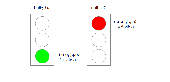
Constraints drum-buffer-rope uses the road runner ethic instead. The analogy is that the road runner (both
fictional and in real life) has just two speeds, fully-on, and fully-off, and
this is how non-constraints should work in drum-buffer-rope. If there is work; work on it at normal
pace, if there isn’t work; don’t work on it.
However, it seems that some people take the cartoon interpretation too
literally and believe it to mean working at more than normal pace. This is not the case. The road runner ethic says just two things; (1) When there is work, complete it promptly. (2) When there is no work, find something else to do. Implementations
get into trouble when there are reluctant road runners. Reluctant road runners are a management or
leadership issue; it is not a worker issue. Another way of
looking at this situation is through the terminology of activation and
utilization (17). Activation at its
most basic interpretation means working for the sake of appearing to be
busy. Utilization means working only
to create or protect throughput. We
saw previously that one of the synchronous manufacturing principles was: Resources must be utilized, not simply activated
(17). This is a re-verbalization of
the need for adequate subordination. If there are
local efficiency measurements still in place then don’t expect to see
roadrunner. Don’t expect to get the
same results either. Implementing
roadrunner while having another older and stronger counter measurement will
cause it to fail. Timesheets broken
down by job or task for non-constraints is a powerful signal to be busy all
the times. Even when the system owner
in such an environment includes a code for “Roadrunner” on the time sheets –
which in effect means “I’m idle” – do not expect to see it used. Believe me. There is quite
an old term used in manufacturing to describe the practice where people work
just as slow as necessary and no faster – soldiering (18). Taylor sought to a large As we reframe
the situation from a reductionist/local optima approach to a systemic/global
optimum approach we must be aware of not only the presence of new
measurements and behaviors, but also of the presence of old measurements
which continue to underline old behaviors.
If you have reluctant roadrunners then look for “legacy” measurements
that are causing that behavior. I have seen
the so-called “laziest” group in a factory embrace roadrunner, and use the
spare time to maintain their gear – something that previously they had been
hard pressed to do. To understand
this, just think back to the section on people. People will make the best decision that
they can based upon their map of reality.
If you change the map of reality you will change the behavior as well. If you measure
people based on local efficiency you will get soldiering – guaranteed. If you measure people globally, you will
get roadrunner – guaranteed. You can “wing”
a large amount of improvement in a process just from improved exploitation
without necessarily utilizing full subordination such as roadrunner. For instance you can obtain impressive and
rapid improvements in output where time sheets are still in force, but the result
will be soldiering in several departments and the illusion within middle
management that it is impossible to improve any further – after all the guys
are fully busy. It really depends
whether we want a process of on-going improvement or a one-off gain. Let’s
complement our understanding of the roadrunner ethic with the traffic light
analogy that we developed in the section on process of change. When a non-constraint is working it is
creating throughput, and when a non-constraint is not working it is creating
protection for throughput.
Batch sizing
is an important part of subordination.
Sufficiently important that we will give it a page of its own. Obtaining agreement to modify batch-size is
a major part of most process implementations. As work-in-process
decreases there are going to be a lot of devices left around that the work
used to sit on and also maybe moved on.
Remove these at a healthy and proactive rate as they become free. If there is somewhere for people to put
work down on, then people will find work to put down on it. When there is insufficient work available
to cover the “empty” spaces people become uncomfortable. Remove the cause of the discomfort – the
empty and unnecessary pallets, trolleys, or what-have-you that is in excess. Clean them up and make sure people know they
have been put away for safe keeping.
We don’t expect to ever use them again; but most others will be
expecting that they will be used again shortly. This way everyone is happy until we all
forget that it was ever an issue. This one
requires patience, persistent patience.
Let’s go back a step or two.
Many drum-buffer-rope implementations will have previously had some
sort of MRP scheduling system in place, or in its absence some sort of
“hands-on” method of expediting. The
whole rationale of the scheduling component of MRP in a job shop or
repetitive batch environment is that it is able to reschedule any process
stage by reprioritizing the sequence that work waits in queues prior to each
stage of the process (21). Drum-buffer-rope
removes the need for queuing everywhere but not the bad habit of
reprioritizing work in the queue. Some
jobs may simply float for a day or two until they are done – continuously
passed by more recent jobs that have arrived.
In cultures where seniority is highly respected, and there are senior
operators, it may be extremely difficult to get first-in-first-out operating
initially. Persist. Because
material is released to the system in the sequence that it will be processed
on the constraint, then in most cases simple first-in-first-out will preserve
the constraint schedule sequence.
Failure to observe this will quickly lead to holes in the buffer. Work that is passed over at a
non-constraint will be detected as late at the buffer. Work that is favored will be detected as
unusually early at the buffer.
Everyone knows which are the “sweet” jobs, if they start to turn up
early then be paranoid. At
non-constraints; “The method of determining priority is first in first out
(FIFO). Since the schedule for the
constraint and the amount of protection required determines the release date,
the sequencing of orders has already been determined and should be by arrival
data/time to the non-constraints.
Unless there is a problem causing an order to penetrate zone one in
buffer management, no effort is made to change this rule (22).” In large
volume conditions however we need to note the following for non-constraints;
“In the case of a shop that has many jobs arriving in a day, a method has to
be devised to determine the sequence in which the jobs arrive. This will dictate the sequence of
processing. The procedure addresses
two things – how to know what arrived first, and how to make sure people work
in that sequence (23).” Even in the
very best systems, occasionally “stuff happens” and we can’t always deliver
on time or ex-stock as we initially promised.
Material shortages are probably the number one cause for this. Over-promising by non-manufacturing
personnel is probably the number two reason.
As a consequence usually the IT guys get given a project to do to
build some meaningful measure of lateness.
Why the IT guys? Well it has
numbers in it and uses the MRP system so it must be an IT job. Of course the IT guys come up against the
age-old problem of whether to measure in units of time or units of sales
value. Do we measure the number of
days late and under-report a big job that was just a day late or do we
measure sales value and under-report the small job that was held up for
several weeks while we waited for a part from the outsourcer? The answer is
that we measure both, using the value of throughput-dollar-days (12). On any given day we multiply any late
order’s throughput by the number of days that it is late and sum for all the
late orders. Of course it should be
zero but sometimes it won’t be. For
orders whose lateness impinge upon our customers we should measure from the
original required delivery date for make-to-order and the order date for
make-to-stock (goods should be availably ex-stock at the time the order is
placed). However, Goldratt suggests
that in order to avoid this most undesirable situation we should also “tie”
the lateness to buffer holes (12). "Sometimes an action by the
organization is triggered due to a deviation in a local department. This occurs whenever a task does not arrive
at its buffer‑origin even though enough time had elapsed since its release,
enough time to cause us, in quite high probability (let's say over 90
percent), to expect the task's arrival.
Thus, we might start to count the days from the point in time when the
task penetrated into the expediting zone, rather than from the order due‑date. This will give us time to correct the
situation before damage to the entire company is fait
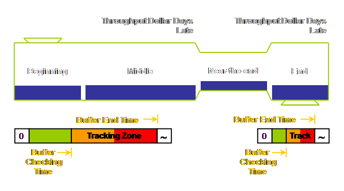
accompli." We might
consider this to be a tactical
application. Thus a work order that is
late to zone 1 of any buffer should have in the buffer report a value for
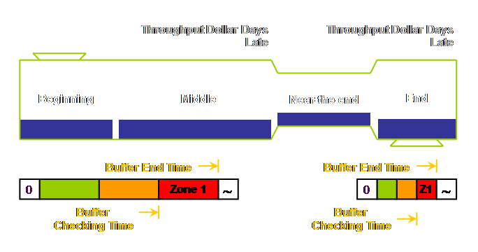
throughput-dollar-days. Let’s draw
that.
Lateness
= Rope Length – One Zone Length – Actual Duration Using the
example from the section on drum-buffer-rope.
Our rope length was 9 days and each buffer zone is 3 days. Therefore any work not at the buffer origin
in (9 - 3 =) 6 days should be located and any apparent cause for the delay
recorded. If the job actually takes
6.5 days then the hole in the buffer is 0.5 days long. Note once
again that the buffer end time, the zone length, and the buffer checking time
are all measures of time which we have drawn in space on our diagram. Viewing buffers like this is a major source
of confusion caused by the limitations of our two dimensional representation. The only
person who needs to know the buffer checking time for a job is the buffer
manager. Don’t add it to the plant
schedule or else it will immediately become an intermediate schedule date and
people will leave work until the last minute – and it will be late. In effect having such a date on the
schedule creates a “concrete” zone 1 buffer in most people’s minds. This is not correct; the buffer extends
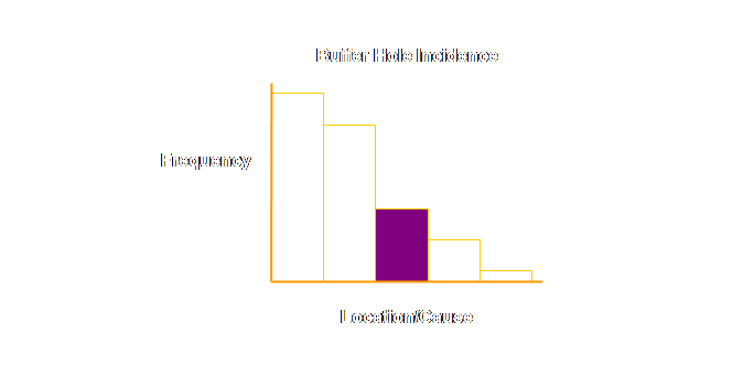
from material release until the scheduled beginning on the constraint. Using buffers
to manage in this way we not only have information on the probable location
of the problem and the frequency of incidence but we also have some measure
of the severity from the system’s viewpoint.
The more days late, and the more throughput at stake, then the more
severe the problem. This information
is currently missing from most buffer reports. Stein advocates exactly this when preparing
a buffer hole Pareto chart (25, 26).
Let’s try and show Stein’s argument graphically. Currently a
Pareto chart of buffer hole incidence might look something like this;
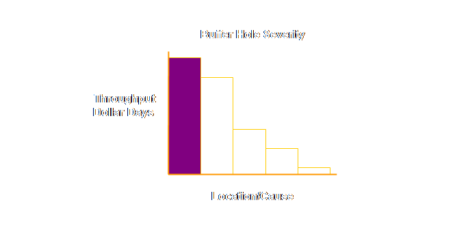
Severity
= Throughput x Lateness This can
change the way that we view the information.
For instance the graph might now look like this;
This is valid
information for the 5-10% of orders that we have to expedite. But what if the order is no longer at the
resource that caused the lateness. How
can we know what to improve in this instance?
The answer comes back that we must deepen the statistic (27). A more satisfactory concept might be that
of a “tracking zone” established expressly for this purpose (27). Stein advocates extending the buffer
checking point out to zone 2 (25, 26).
It is now far more likely that an order will be found at the location
that is causing it to be “late” and it is also far more likely that emergent
problems will be found before they become critical. We might view this to be a strategic application of buffer management. Let’s draw that.
Tracking
Hole = Rope Length – Two Zone Lengths – Actual Duration Again using
the example from the section on drum-buffer-rope. Our rope length was 9 days and each buffer
zone is 3 days. Therefore any work not
at the buffer origin in (9 - 3 - 3 =) 3 days should be tracked and its
location recorded. If the job actually
takes 4.5 days then the tracking hole is 1.5 days long. I don’t think
the intent is that tracking should be undertaken for every job, even though
our manufacturing system might be able to show us every hole in the tracking
zone. It is unlikely however that we
will know where the job is without physical inspection, and so this type of
data analysis should be periodic at best – sampling the system performance
from time to time in other words. A process is
like a sponge; we go about squeezing the excess work-in-process out of it,
then let it rebound to its original shape and put it back down on the
bench. WARNING, if there is any water
on the bench the sponge will simply soak it up again. If you don’t have the vigilance of a hawk
your system will start to build inventory as soon as possible. The previous best way to keep a tag on this
is either by a measure of work-in-process or a measure of lead time.
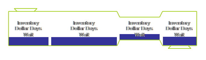
Moreover, as a
drum-buffer-rope implementation begins to give increased sales the volume of
work in the process will have to increase unless the rate of flow (the lead
time) decreases. Use
inventory-dollar-days as a way of continually driving the system to better
levels of performance. Don’t let the
value rise because it indicates that your process is becoming slower –
customers don’t like that. At a
departmental level, inventory-dollar-days is a good way to keep a handle on
aging work if sweet jobs are queue jumping other jobs. Failing this, then at least have a daily
graph of local work-in-process versus output.
From this you can derive an indication of local departmental lead
time. Why do this? Well, as work-in-process goes down, people
often slow down too. This graph will
focus on the positive of the decreasing lead time and warn whenever it is rising. It also removes the focus from the total
work-in-process. Remember that maybe
just a few weeks earlier a large work-in-process was a measure of how busy
and important a department was. We
have to replace that measure of importance with another – short lead times. The concept of
a buffer manager is pivotal to the smooth execution of drum-buffer-rope. The actual person who occupies the position
will depend upon the size of the firm.
For a small firm the buffer manager may well be the owner or a foreman
– indeed the foreman if the firm is not too large. In larger firms it might be a senior
planner or the production manager.
Whoever it is, they must have the vested authority to determine the
priority of work in the non-constraint areas. Buffer
management has two functions which we have seen; strategic
and tactical. The tactical function is to enable the
limited expediting of jobs that might not otherwise reach the constraint on
time. The strategic use is to monitor
the size of the buffer and conversely the aggregate sprint capacity of the
non-constraints. This will identify
potential emergent constraints. We now
have sufficient system-wide vision to decide whether to invest in additional
capacity, or better subordination, or longer buffers. Buffer
management reporting is the subordination control mechanism that replaces
legacy efficiency reporting. Buffer management reporting is a replacement, not
an add-on mechanism (29).
“If anyone
adjusts a stable process to try to compensate for a result that is
undesirable, or for a result that is extra good, the output that follows will
be worse than if he had left the process alone (3).” The process of interfering in a stable system
is often known as tampering. It is the
epitome of a combination of people wanting to do their best, and the effects
of dynamic complexity. A local action
(in time) that is perceived to be positive may have negative ramifications
for the system as a whole at some later time.
We mentioned the impact of this – the failure to “learn from
experience” in the introduction. Essentially
the stages of identification, exploitation, and subordination seek to
stabilize the system around the goal, usually maximal throughput in
manufacturing or output in a not-for-profit organization. Be careful however, just because you have
removed expediting from the shop floor for instance, there will be other
people who will “tamper” with the resulting stable drum-buffer-rope process
with the best of intents. However they
will cause harm. Again it arises from
failure to learn from experience because the feedback is blocked by distance
and time. Consider for a
moment the example where the sales function “forgets” to tell manufacturing
about a promotion in good time – has that ever happened? And then the sales function panics and
interferes with the schedule. Sales
meet their short term objective of getting additional promotional stock, but
harm other orders. It is much better
to allow the buffer manager to deal with the problem as best possible within
the existing system. It is absolutely
essential that the harm caused by tampering is highlighted to everyone. Better still make sure the holistic
approach has been used so that all parts of the process are aware of the
constraint and the effect of tampering before the implementation begins. Elevation is
so system specific that it isn’t possible to address it here. It may however be some considerable time
until we need to elevate if the exploitation and subordination stages are
approached as a true process of on-going improvement. If a
constraint is elevated sufficiently that it is broken, then we must go back
to the first step and identify the next constraint. Well, that is if we are not to allow
inertia to take over as satisfaction with the current status. Of course we would expect that buffer
management would have identified the next physical constraint. It may not however adequately identify the
policy constraints that give rise to physical constraints. So we shouldn’t forget to expose our
investigation to the rigors of the Thinking Process current reality tree when
we begin to identify a new constraint. There is
another aspect to this stage of the process.
We can make it quite proactive rather than passive by selecting a
strategic constraint. Indeed as
knowledge of the way the business generates throughput or output improves it
is very likely that a strategic constraint will be selected and managed. Let’s look at this further. In the first
stages of an implementation people are going to raise the issue of “if we
exploit this constraint, we may in fact elevate it above something else and
the constraint will move to there.”
“AND if we begin to exploit the new constraint, it too, might be
elevated above something else and the constraint will move once again.” Exactly right. It could sound
like a weak excuse to do nothing, in reality it is peoples’ intuition telling
them that, yes, if we know where to focus we can break constraints
easily. And at the same time that same
intuition is telling people that they really don’t know where the next
constraint will be and with that there is a feeling of powerlessness or loss
of control. After we begin
to dry a process out we can begin to make conscious decisions about where we,
the management, want the constraint to be.
In effect we are choosing a strategic constraint; we are making a
decision to always build sprint capacity ahead of building capacity on the
constraint. There are good reasons for
this. The constraint dictates the way
in which the firm will make money – and capital investment, product
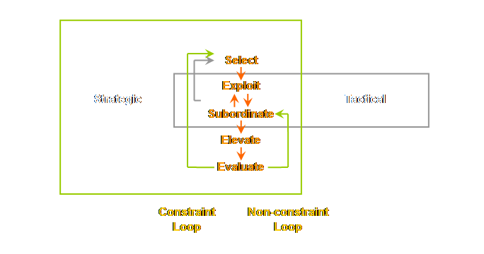
development, marketing and sales. Newbold, using
the language of leverage points rather than constraints; reworded the 5
focusing steps to accommodate this strategic perspective (30). (1) Select the leverage points. (2) Exploit the leverage points. (3) Subordinate everything else to the above
decision. (4) Elevate the leverage points. (5) Before making any significant changes, Evaluate whether the leverage points
will and should stay the same. The new key
words are; select and evaluate. This requires
a more focused approach to non-constraints and near-capacity constraints. Near-capacity resources must be removed
(30). Therefore; (1) Identify near-capacity constraints. (2) Evaluate their significance. (3) If necessary, remove their impact. Essential this
is a type of “subroutine” loop for near-capacity constraints running within
the subordination step above. We drew
this on a sub-page off the page on evaluating change. Let’s draw a similar diagram here.
The
identification and evaluation of near-capacity constraints is of course a
strategic function of buffer management.
Using the tracking zone from time to time will help to answer these
strategic questions. Don’t ever
underestimate the power of being on the floor or wherever the real work is
done. Things will go wrong. You will be able to solve problems with
direct management involvement in 15 minutes on the floor that you will not
have been able to solve with the same management in 55 minutes of “office”
meetings. Let’s repeat a
useful trinity from the beginning of this page. Go to
the actual place See the
actual problem Talk to
the actual people If you can’t
do this with the management then you are being stonewalled. Don’t worry, the management will be
surprised at the new found speed of problem resolution and will grow to like
it. Where does
this trinity come from? Well, I learnt
it from TQM but could never track the source down despite the smoking gun of
Ohno’s admonishment to stand all day until you understand the flow of the
process. It does, however, indeed come
from Toyota and is a verbalization of the Toyota principle of genchi genbutsu (31).
It is really an acknowledgement that the required knowledge can only
be gained tacitly rather than explicitly. We have seen
in the previous section the basics of drum-buffer-rope. In this section we have seen some
additional implementation detail.
However, there are some issues that need to be addressed further. Therefore, over the next 4 pages we will look
at; batch issues, quality, alignment, and the time required for implementation. Let’s have a
look at batch issues next. (1) Ohno, T.,
(1978) The Toyota production system: beyond large-scale production. English Translation 1988, Productivity
Press, pg 78. (2) Woeppel.
M. J., (2001) Manufacturer’s guide to implementing the Theory of
Constraints. St. Lucie Press, pg 87. (3) Deming, W.
E., (1982) Out of the crisis.
Massachusetts Institute of Technology, pg 327. (4) Goldratt,
E. M., (1990) The
haystack syndrome: sifting information out of the data ocean. North River Press, pg 131. (5) Caspari, J. A., and Caspari, P., (2004) Management Dynamics: merging
constraints accounting to drive improvement.
John Wiley & Sons Inc., pg 180. (6)
Schragenheim, E., and Dettmer, H. W., (2000) Manufacturing at warp speed:
optimizing supply chain financial performance. The St. Lucie Press, pg 124. (7) Stein, R.
E., (1996) Re-engineering the manufacturing system: applying the theory of
constraints (TOC). Marcel Dekker, pp
112-115. (8) Caspari,
J. A., and Caspari, P., (2004) Management Dynamics: merging constraints
accounting to drive improvement. John
Wiley & Sons Inc., pg 175. (9) Woeppel.
M. J., (2001) Manufacturer’s guide to implementing the Theory of
Constraints. St. Lucie Press, pg 140. (10) Cox, J.
F., and Spencer, M. S., (1997) The constraints management handbook. St Lucie Press, pg 86-87. (11) Umble,
M., and Srikanth, M. L, (1996) Synchronous manufacturing: principles for
world-class excellence. Spectrum
Publishing, pp 186. (12) Goldratt,
E. M., (1990) The haystack
syndrome: sifting information out of the data ocean. North River Press, pp 146-155. (13) Smith,
D., (2000) The measurement nightmare: how the theory of constraints can
resolve conflicting strategies, policies, and measures. St Lucie Press/APICS series on constraint
management, pg 67. (14) Smith,
D., (unpublished) Gain more speed and predictability through adequate
protective capacity. Chesapeake
Consulting Inc., 4 pp. (15)
Schragenheim, E., and Dettmer, H. W., (2000) Manufacturing at warp speed:
optimizing supply chain financial performance. The St. Lucie Press, pg 175-176. (16) Kawase,
T., (2001) Human-centered problem-solving: the management of
improvements. Asian Productivity
Organization, pg 111-119. (17) Umble,
M., and Srikanth, M. L, (1996) Synchronous manufacturing: principles for
world-class excellence. Spectrum
Publishing, pg 74. (18) Kanigel, R., (1997) The one best
way: Frederick Winslow Taylor and the enigma of efficiency. Viking, pp 141-142, 163-166, & 203-210. (19) Goldratt, E. M. (1996) Production the TOC way,
Tutor guide. Avraham Y. Goldratt
Institute, pp 46-48. (20) Goldratt, E.
M., (1990) The
haystack syndrome: sifting information out of the data ocean. North River Press, pp 88-89. (21) Cox, J.
F., and Spencer, M. S., (1997) The constraints management handbook. St Lucie Press, pg 90-91. (22) Stein, R. E., (1994) The next phase of
total quality management: TQM II and the focus on profitability. Marcel Dekker, pp 99-100. (23) Woeppel.
M. J., (2001) Manufacturer’s guide to implementing the Theory of
Constraints. St. Lucie Press, pp
128-129. (24) Goldratt,
E. M., (1990) The
haystack syndrome: sifting information out of the data ocean. North River Press, pp 130 & 129. (25)
Stein,
R. E., (1994) The next phase of total quality management: TQM II and the
focus on profitability. Marcel Dekker,
pp 92-99. (26) Stein, R.
E., (1996) Re-engineering the manufacturing system: applying the theory of
constraints (TOC). Marcel Dekker, pp
141-151. (27) Goldratt,
E. M., (1990) The
haystack syndrome: sifting information out of the data ocean. North River Press, pp 139-140. (28) Goldratt,
E. M., (1990) Essays on the Theory of Constraints, Chapter 3. North River Press. (29) Caspari,
J. A., and Caspari, P., (2004) Management Dynamics: merging constraints
accounting to drive improvement. John
Wiley & Sons Inc., pp 187-188. (30) Newbold,
R. C., (1998) Project management in the fast lane: applying the Theory of
Constraints. St. Lucie Press, pp
152-155. (31) Liker, J.
K., (2004) The Toyota Way: 14 management principles from the world’s greatest
manufacturer. McGraw-Hill, pp 223-236. This Webpage Copyright © 2003-2009 by Dr K. J.
Youngman |