|
A Guide to Implementing the Theory of
Constraints (TOC) |
|||||
|
Multi-Project Drums |
|
|
|
Comparing
Safety In Production & Projects There are two
groups of people who are likely to use these pages on projects; those with
prior knowledge of production operations (manufacturing) and those with pure
project backgrounds. For this reason I
want to compare and contrast between production operations and project
operations. The similarities are much
greater than the differences. I want
to do this for two reasons; 1. Provide a bridge for people with production operation experience in
order to enter into the project domain. 2. Show people with project operation experience that the challenges that
they face are not that different from those experienced in production
environments. So I ask for
your indulgence if you already feel slighted that “your” area of expertise is
apparently no more difficult than “their” area of expertise. You see, we are basically all in the same
boat – and we are all at sea as well.
Industrialization is new. We only have to
check whether our parents’ generation ran projects or production operations
as we do, and if they did, then check out our grand-parents generation. The scale and scope of operations today is
vastly different from that of just one or two generations ago. For instance, just one generation ago we
didn’t have computers to make mistakes quite as quickly as we are able to
today. In fact,
computers are now so ubiquitous that we can discuss operations in terms of
the software that drives them, or at least the generic approaches. For production operations the first
software was material requirements planning (mrp or small mrp – referring to
the use of lower case letters).
Material requirements planning allowed the building of bills of
material (BOMs) for a process; a list of all the bits and pieces and maybe
the places where, and the time when, they were required. It wasn’t long before this was beefed up to
materials resources planning (MRP or MRP II) with the addition of capacity
scheduling of each step in the routing that had been used to generate the
bill of materials. More recently this
has been beefed up once again to enterprise resources planning (ERP) where
schedules are wired across functions as well as within functions. Sales and marketing now know what
production is doing and vice versa (well it sounds good doesn’t it?) The project
operations equivalent of the mrp, MRP II, ERP, alphabet soup is Critical Path
Method, (CPM for short). Critical Path
Method tends to be associated with the Gantt charts that are used to
graphically present the relationships between tasks in a project, but it is
generated from an approach called program evaluation and review technique (or
PERT for short). In fact, as we will
soon see, program evaluation and review technique can be equally applied to
production operations as well as to projects.
Indeed, maybe PERT is responsible for the two short comings of both
MRP and CPM. Both approaches assume,
even today, that there is more capacity at each step in a production process,
or task of a project, than is actually required. Colloquially, we tend to call this
“infinite capacity” although we only mean that there is “more than
enough.” Before the advent of
computers when PERT was a manual exercise, this simplification made the
impossible possible. Also, both MRP
and CPM assume that safety is localized throughout the respective
operations. In production operations,
safety is localized in the queuing of product (work-in-process). Each queue represents a safety buffer that
allows late work to catch up to its schedule through the rearrangement of items
or “jobs” in the queue. Historically,
these types of scheduling approaches originated in so-called job shop
environments – places where machinery was likely to be grouped according to
function, rather than the flow-shops that are so much more common in all but
the smallest of facilities today. In
Critical Path Method the safety is localized not in the queue, but within
each and every task in the project. Assumptions of
infinite capacity and the localization of safety throughout the operation are
the two aspects that cause so much trouble to modern operations. We won’t address the issues of infinite
capacity assumptions until the next page on Critical Chain Project
Management, because this is an important issue of itself and is to me the
distinction between Critical Chain Project Management and Critical Path
Method. On this page we will address
the issue of localized safety in each step or each task. Essentially we are going to move from
safety that is localized, specific, and everywhere, to safety that is
general, aggregate, and located in just a few critical places. Having safety
“embedded” in each step of a production process or each task of a project
ought, at first pass, seem to be an effective solution. After all you can size each individual allocation
as required – regardless of whether it is explicit within a production
process queue, or implicit within a project task. However, a number of operational and
psychological factors contrive against us.
The operational factors are the dependent nature of serial operations
and the inherent variability that occurs within each operation. The psychological factors are varied, and
probably more important for project-based operations than production-based
operations. We will deal with the
psychological factors as we come to them. In order to
develop the argument for the aggregation and placement of buffers in project
management, I am going to use a PERT diagram for both a production process
and a project. In order to do that we
must make use of the realization that a project is an “A” plant tipped on its
side. Let’s look at
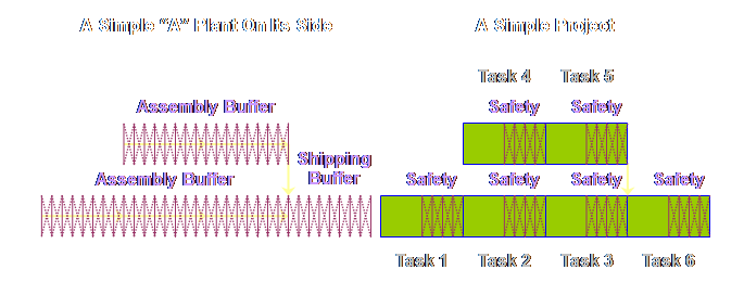
this in more detail. A project is
an “A” plant tipped on its side (1).
This is the “thing” that finally allowed me to see the relationship
between production operations and project operations and their buffers or
safety. But what is an “A” plant you
are asking? Theory of Constraints sees
4 generic flows in production operations, they are; “V” plants or divergent
plants (divergent from the bottom of the “v” to the top), “A” plants or
convergent plants (convergent from the bottom of the “a” to the top), “I”
plants or linear plants, and “T” plants – a plant with a linear stem and an
explosion of choices at the top (assembly).
Each type of plant is typical of particular operations. “A” plants are typical of situations where
a number of different components from different raw materials come together
to form a final assembly. Let’s draw a
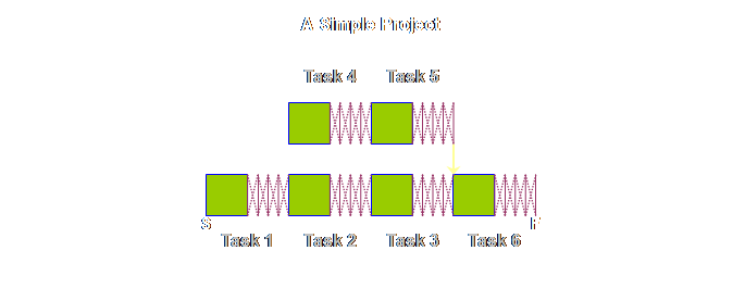
simple, a very simple, “A” plant on its side to see how it would look.
This type of
logic diagram is common in Theory of Constraints. The logic might coincide with the physical
layout of the plant; more often than not, it won’t. For an example of a more complex “A” plant
logic diagram and its corresponding physical layout, have a look at the
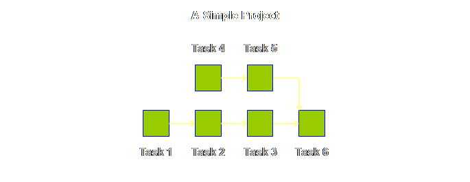
diagrams for the P&Q Question. If we were to draw
a very simple project, then apart from some different names, it would look
exactly the same, lets see.
The logic
diagram for production operations and project operations are exactly the
same, save for different labels. Let’s
put the two diagrams side-by-side.
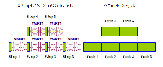
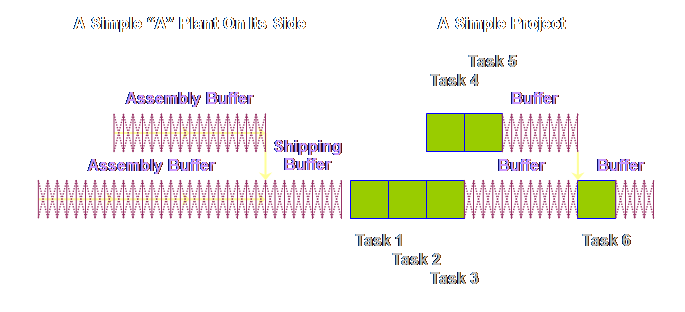
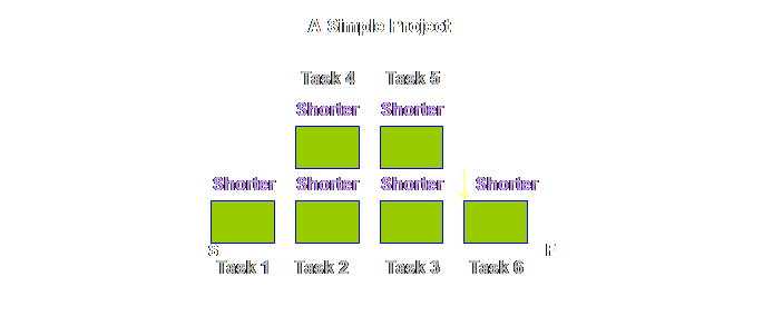
Let’s draw
each respective diagram so that the steps and tasks are somewhat proportional
to the time taken.
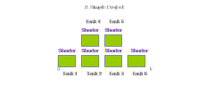
Let’s have a
look at this waiting in queues.
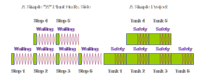
This raises a
question; there isn’t any waiting in projects – right? Well, not explicitly, and it isn’t called
waiting, it is called safety – “things” in production might wait but people
in projects don’t like to be seen waiting, so we have to call it safety. Let’s have a
look.
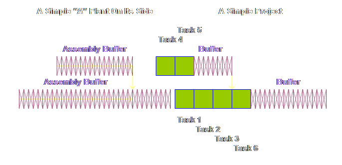
Having got
this far (even if you really don’t think that there is any safety in projects
what-so-ever), we can now show the apparent differences between buffering in
production operations in Theory of Constraints and buffering in project
operations in Theory of Constraints.
If buffering is an unfamiliar concept to you, then please wait a short
while. We need to bury the devil which
says that buffering in the two approaches is different. Once we have done that, then we can start
all over again with the vexed question of why we even have buffers in project
management. Let’s start
first with our “A” plant process. What
if we accept that we can move from an MRP schedule to a drum-buffer-rope
(DBR) sequence. In drum-buffer-rope
the only things scheduled are the start and the finish (and maybe the drum
but we will leave that out here). If
we accept that, then we can aggregate the touch time and we can aggregate the
waiting time. By aggregating the
waiting time we make the total waiting time available to the whole process. Let’s have a
look.
What happens next is that because the touch time in production
operations is so small (remember we have drawn it here 1 to 5 to 10 times too
large) it is ignored completely. This is what our process looks like as a consequence.
What then if
we accept that we can move from a Critical Path schedule to a Critical Chain
sequence. The only things scheduled
being the start and the finish. If we
accept that, then we can aggregate the touch time and we can aggregate the
safety time. By aggregating the safety
time we make the total safety time available to the whole process. Let’s have a
look.
Having made
these changes, do you see the apparent difference between the two sets of
buffers? To me, the buffers in
production operations appeared to occupy the whole of the process. In project operations the buffers don’t
occupy the whole of the project, instead they appear to be bunched-up towards
the end. However, the reality rather
than the appearance is more important.
The reality is that the buffers in both cases are treated in exactly
the same way, the only difference is that in one of the cases, production
operations, we can make a simplifying assumption and remove the touch time
from contention. That is all that we
have done that is different. The exact
mechanics in each case are a little different from this simple example. We have dealt with the production
operations case in detail in the production pages of this website, and we
will deal with the detail of project operations case over the remainder of
these project pages. Although the
detail may vary, the principle is the same (and in distribution and raw
material supply as well); we wish to identify and locate all the locally
distributed safety or waiting and aggregate it into one or several
strategically placed global buffers where the least total safety can be of the
greatest benefit to the system as a whole.
If we can remove safety that is embedded but wasted then we should be
able shorten the duration of the project without endangering the on-time
reliability of the completion date. In
fact, as we will see, we can substantially improve the reliability of the
completion date as a consequence. First,
however, let’s consider a few more aspects of touch time and variability in
production operations and projects. The touch time
in production operations is a very small part of the total time spent in the
process; most of the time is, in fact, spent waiting. In addition to the touch time being a small
part of the total, there is also little variability in its duration. This isn’t so much a case of the
repeatability of the tasks, but rather the mechanization of the tasks –
although, clearly, the more often a task is repeated the more likely we are
to want to mechanize it. And if we can
mechanize it, then automation is the next logical step after that. There are without doubt some manufacturing
tasks which have greater variability in their touch time than others; those
that use natural products and those that use manual labor are the two that
spring to mind. However, even in these
cases the variability is still not large. So where then
is the variability in production operations?
It is in the wait or queue time?
In fact, it is an assertion. I
can’t quantify the assertion because I have never seen a graph of variability
in wait time. There is genuine concern
about the amount of work-in-process and hence total wait time in a process,
but little interest in its variability between the same steps for the same
product. Its an invisible attribute. What then of
projects? Let’s start at the easy
place. Variability in wait time or
safety time is said to not exist, because safety time is said not to exist,
or at least insufficient safety time is said to exist because some tasks in
projects, and certainly almost all whole projects, tend to be late rather
than on-time or even early. In the
first instance then, it is better to view a project as a mirror image of a
production process. All the
variability in a project appears to be in the touch time of the task. Why should the
touch time of a task be variable? To
answer that we have to look at two things; § The nature of the task § The nature of the resources (= people) Let’s look at
the nature of the task first, and let’s just limit ourselves for the time
being to the realization that sometimes the subject matter of the task
unfolds swimmingly well, and equally, sometimes it does not. Thus there is some natural variability even
if a particular task is well known and well practiced. How about the
nature of the resources then? Just as
in production operations, people add variability to a task as well; people
unlike machines have good days and bad days (although I know a few machines
that seemed to be able to mimic this attribute well). If someone has not done a specific task
before, or the task is significantly different from prior experience, then we
ought to expect greater variability.
The task may take less time, it may take more. People with a large amount of prior
experience (both explicit and tacit knowledge) might turn out less variable
results than someone who is new. Let’s
summarize this. There
is variability around what is known Even if we
confine ourselves to what is known within the task of a project, then there
is variability. Because the touch time
is so large in proportion to the duration of the whole project, so too, is
the effect of any variability. In
production operations the task variability is small, the tasks are small, and
the shock absorbers for this, the in-queue waiting time, is huge. In project operations in contrast, the
tasks are large, the variability is therefore magnified, and the shock
absorbers are perceived to be small to non-existent. Let’s confine
ourselves for the moment to just this simple view of task variation. It is naive I know, but if we can understand
the effects in this simple case, then the more complicated issues caused by
uncertainty will fall out as a consequence.
We will address uncertainty, but not quite yet. Let’s have a look at the effect of
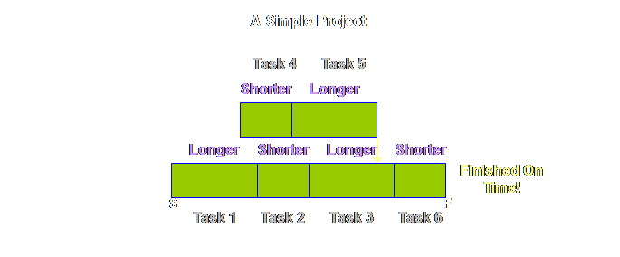
variability on dependent tasks in a simple project. Common sense
would seem to suggest to us that variability in project tasks ought not to be
such a bad thing. Surely over a number
of tasks the variability should average out?
Surely the larger the size of a project, and the number of individual
tasks, the more likely it is that the project will come in on time as the
over-runs and under-runs average out? If this is our
plan,
Sad, is it
not? But it gets worse. Let’s see.
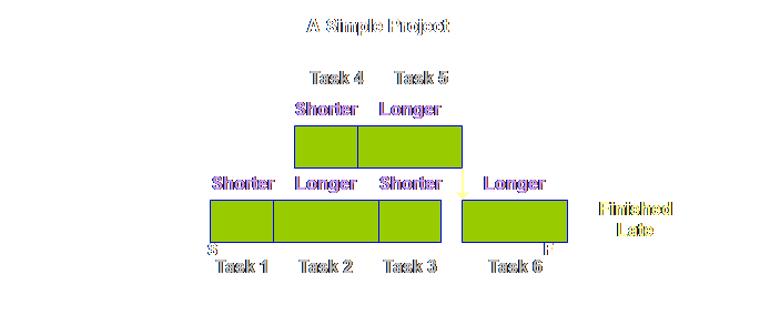
Multiple
dependency at convergences have quite an impact, but there are also other
dependencies wherever there is a “hand-off” between two adjacent tasks. We might not like to think of them in the
same terms as the convergence, but alas, the mechanics are exactly the
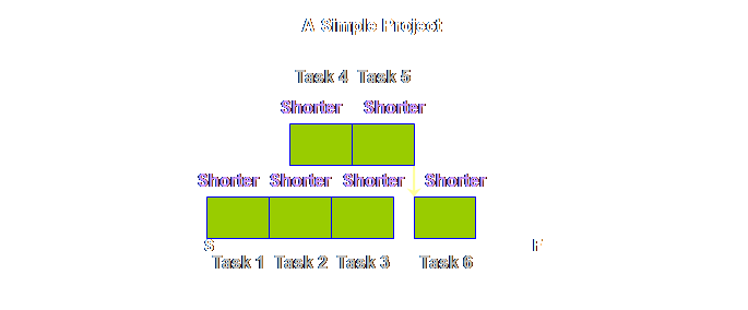
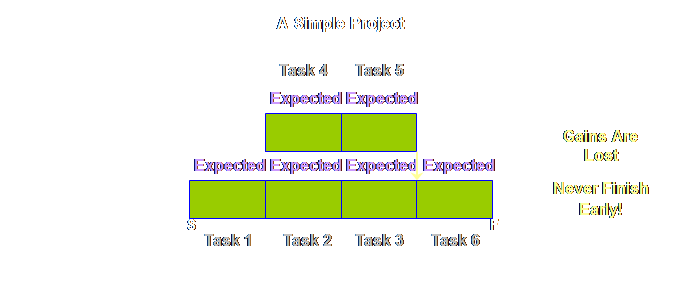
same. Let’s have a look. Let’s take an
extreme example where all of the tasks are completed in a shorter duration
than the estimate. The whole project
should finish early – right? If
everything went swimmingly well then this is what we should achieve.
The reasons
that we don’t get early starts to tasks and therefore early completions of
the whole project are manifold. Some
are mechanical, some are psychological (and real rather than imagined). Let’s have a look at the mechanical aspects
first.
If those are
the mechanical reasons (essentially people are busy), what are the psychological
reasons? The psychological reasons
belong more with the early finish of the preceding task rather than the early
start of the succeeding task. Ask
yourself; how often have you seen a task finish early? Probably not very often. Note, I didn’t say ask how often they do
finish early, I asked how often do you actually see it. You don’t see it because it is hidden. It is hidden for a number reasons. In reality we see the following.
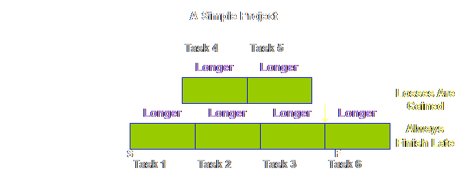
Why would
people choose to slow down their task rather than to complete it early? One sound reason would be to protect the
very valuable safety time that has been so hard fought for and won on
previous occasions and which painful experience tell us that we need more
often than we don’t need. To lose that
safety now would put further tasks in future projects in jeopardy and that is
not something people wish to do at all. The
combination of successor task resources not being ready to start early when
there is an early finish, and predecessor task resources not being willing to
jeopardize future safety by finishing early ensures that gains in
individual tasks are lost and that whole projects never finish early. It sounds like a bold assertion, but I am
willing to entertain any evidence to the contrary. But this is
only half the story. We have only
looked at the extreme of tasks that are shorter than the expected duration
and thus have early finishes. What
about the other direction? What about
tasks that are longer than the expected duration or those that have late
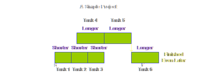
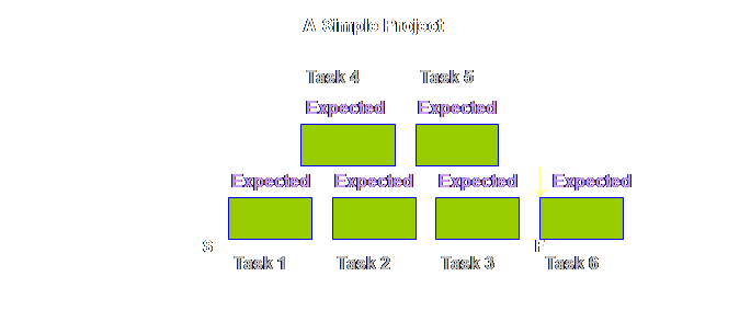
starts? Let’s see. It’s not nice. We start once
again with our simple project with our boringly uniform expected durations
and 6 simple tasks
How about less
legitimate reasons? Well, like the
early finish, we are unlikely to see such late starts recorded. Instead we are much more likely to see the
following.
Its a sobering
effect. We are just trying to do our
best, and yet it seems that at best our gains in individual tasks are lost
and whole projects will never finish early and at worst losses in
individual tasks are gained and whole projects will always finish late. Why do we put
up with this state of affairs? As we saw
earlier, shorter than estimated tasks can average out longer than estimated
tasks, and for that matter early finishes can average out late starts as
well. However, for a number of
mechanistic and psychological reasons this fails to happen. It fails to happen because safety is
embedded in each local task. If for
any reason we fail to utilize that safety it is lost to us for all time. If only the safety was available
in-totality somewhere to share out, rather than being embedded in each local
task, then surely we could resolve the mechanistic problems and maybe some of
the psychological ones too? The only
way to achieve this is to employ global buffering of the project. There is another reason why we must employ global buffering, an issue that so far we have
managed to avoid – uncertainty. So far we have
only looked at dependency in terms of how the completion of one task affects
the start of the next task. Successor
tasks are not only dependent upon the completion of the predecessor tasks,
they are also often contingent upon them.
That is, the nature of the successor task can not be fully determined
until the uncertainty is resolved by the predecessor task. This of course might only unveil further
uncertainty in the current task which is yet to be quantified. For example, a
project that includes foundation earthworks might encounter more difficult
ground or easier ground than prior testing had indicated. Outdoor projects are often contingent upon
the weather. This must be factored
in. Any form of overhaul and
maintenance project is contingent upon the condition of the equipment as
found after stripping the equipment down.
While our local garage may be able to say “it will depend upon what we
find,” project-sized operations must make a reasonable allowance for such
things ahead of the fact. Contingent
dependency and therefore uncertainty are common factors in projects. What happens
the first time a pharmaceutical company makes its first scaling-up experiments? A new recipe that works perfectly in lab
scale trials is moved for the first time to pre-production trials. Sure the rigs are the same as all the other
pre-production trials and yet there is novelty in the current mix. The chemistry, the quantities, the order of
mixing, the mixing itself, and the consequent “cooking” are all new. Will the yield and the quality be
sufficient? If not, what needs to be
changed, and if there is a change, how many more trials until we can bring
the project to market? Where there is
novelty, there is uncertainty. In
fact, where there are unknowns, there is uncertainty. There is one
more major source of uncertainty.
Let’s have a look. In a single
project environment resources may not be dedicated solely to the project
tasks. In many small businesses some
people assigned to project tasks may also be assigned to other non-project
tasks that must be fulfilled, such as day-to-day business or managerial functions. Such a case is very common in smaller
professional firms. In many firms,
both small and large, there may also be many concurrent fee-earning projects
each with its own needs and priorities.
Some people assigned to project tasks may be assigned to multiple
tasks in different projects (and some non-project ones as well). This would not be an issue if each task
could be carried out to completion before the next is started. Reality is that staff must chop and change
– multi-task – between different projects according to ever changing needs,
priorities, and mis-synchronization.
In fact, like fire-fighting in production operations, we often laud
such activity, even if it is to the detriment of the individuals concerned –
they get worn out – and the projects themselves – they are always longer and
later than we want. Uncertainty is
a dominant characteristic of project operations. If we found
that; There
is variability around what is known Then we must
conclude that; There
is uncertainty around what is unknown Unknowns and
the consequent uncertainty are a fact of life in project operations. How do we accommodate such
uncertainty? As it turns out, rather
well actually, lets see. Strange as it
may seem, it is very hard to find a novice production operation; even a new
firm on a “green fields” site that starts from scratch will endeavor to
employ people who have prior experience in the field, especially the detail
complexity of the specific endeavor.
Ditto, project operations. We
know uncertainty exists and we accommodate it by extending the duration of
the individual tasks. The more
uncertain we are, the more likely we are to seek longer task durations. The duration is weighed-up against prior
experience. Every task automatically
compensates or accommodates the uncertainty into the task estimate. The real issue, as with the case of simple
variation, is the existence of dependencies, and the local locking in of the
embedded safety. Greater uncertainty
simply compounds all the effects that we observed earlier due to dependency –
either mechanistic or psychological; any gains from individual tasks are lost
and projects simply don’t finish early.
Moreover, any losses in individual tasks are accumulated and projects
finish later and later. This need not
happen. There is more than adequate
safety allocated and embedded into each of the individual tasks. We started our
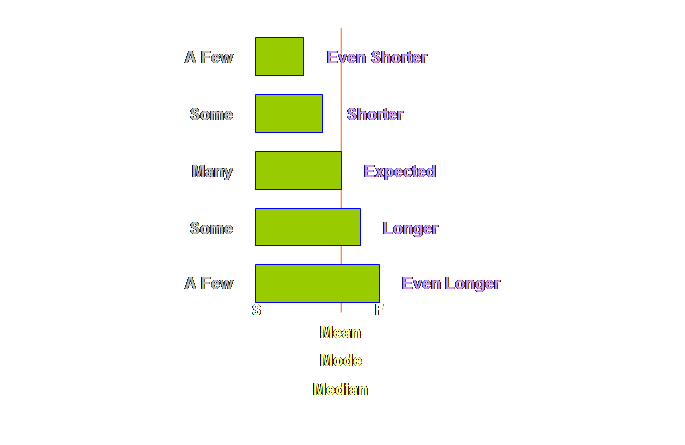
discussion on variability and dependent events with a simple project where
the under-runs and over-runs around an average task estimate cancelled one
another out and the overall effect was that the project finished on
time. This was based in part on the
notion that some sort of “normal” distribution is at work at the task
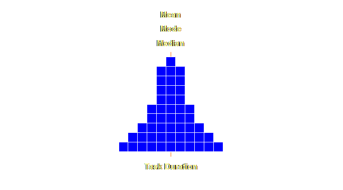
duration level. Let’s have a
look at this.
Let’s expand
this out a little more, a few more extreme values at either end and some
quantitative estimates as well.
Let’s have a
look at this.
Let’s add some
values to this distribution.
We embed the
necessary safety within each and every individual task duration
estimate. However, because this safety
is localized it is frequently wasted and our worst fears come true (again);
the overall project will not be completed on time. We view this as a vicious cycle of a
never-ending need for greater and greater safety estimates within the task
duration. If we could
make this localized safety accessible for any and all tasks within the
project by using buffers, then we would actually need less safety overall and
yet still finish on time. We need to
know how to access this safety, where to put it, and how much. These are essentially our task and buffer
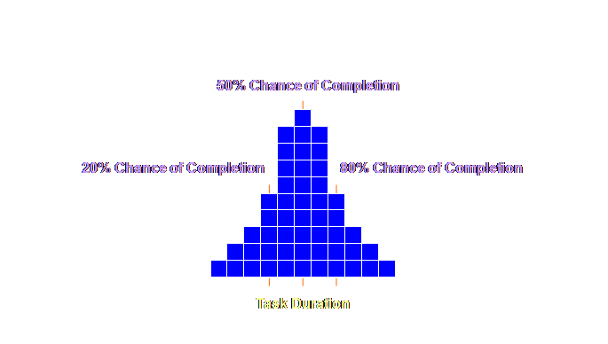
sizing rules. Let’s have a look. Buffer sizing
for projects, as for production operations, is based upon a rule of thumb, a
heuristic if that sounds better. It is
based upon a rule of thumb because this has been found to be thoroughly
effective over a very wide range of scope and scale of project management –
from the maintenance of jumbo sized commercial aircraft to the product
development of the tiny hard drives in our computers (5). Remember we are after effective and
implementable solutions; we don’t want ineffective nor un-implementable
solutions; the world is awash with those already. Let’s have a
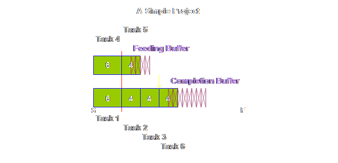
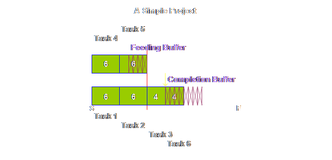
look at the rule. We take our
initial project plan,
By halving the
task duration we bring it back to something around the 50% level. Then we will further protect this with
adequate buffers. This is ample
sufficiency as we will see. The
over-runs and under-runs around this estimate will average out due to the placement
of the buffers. Moreover, halving the
task duration has an important psychological effect that must not be
underestimated in its overall importance.
It stops the waste of unreported early finishes – because there is
precious little time to waste – and it stops the procrastination that causes
late starts – for the very same reason. Some
terminology. This shortened task time
has a number of names, it has been called the “trimmed task time” (4), “best
estimate” or “50% probable” (6). It is
also referred to as the “50% estimate,” the “focused task time,” and the
“reduced task time.” Take your pick. The reason
that there is more than ample sufficiency for individual tasks even at the
50% estimate is because we aggregate
the other half of the task, our safety, at the end of the tasks were it is
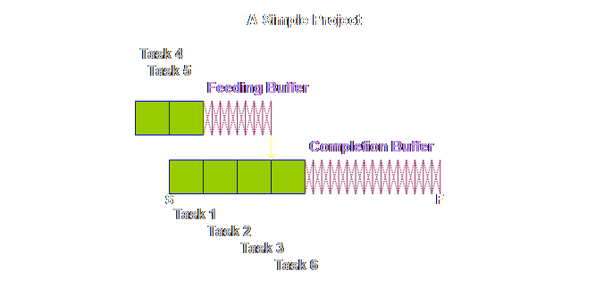
accessible to all of the preceding tasks. Let’s show
this.
Again, we have
some new terminology. The buffer on
the critical chain was initially called the “project buffer” (4) and this
terminology has continued to be used in a number of sources. However, a second term is also in use, that
of “completion buffer” (7). Once again
you can take your pick, however, here we will be using “completion buffers”
because that is what we are buffering and it is good to constantly remind
people on projects that the project will be completed within the completion
buffer – the term is self-reinforcing.
The feeding chains that arise parallel to the critical chain are
uniformly called “feeding buffers.” It is probably
better to keep the name “project buffer” as the name of the class, and
“completion buffer” and “feeding buffer” as members of the class, just as
buffers in production operations consist of drum buffers, assembly buffers,
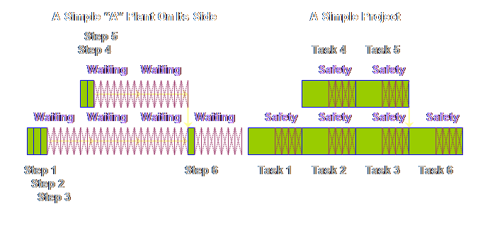
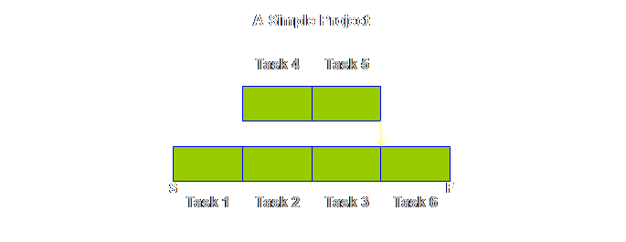
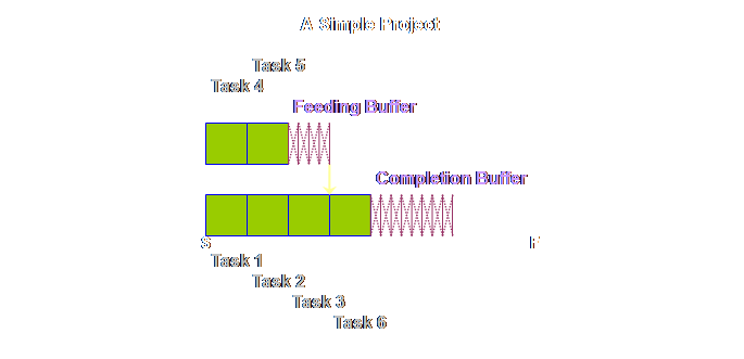
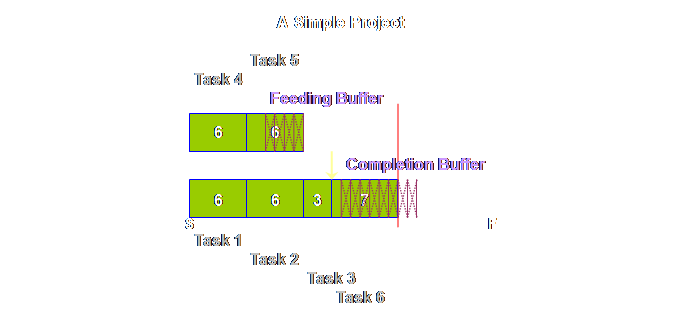
and shipping buffers. Returning to
the detail of our simple project above, once again we find that tasks 4 &
5 are pushed back and that this has increased the total length of the
project. However, this is just an
intermediate step. Because the local
safety is now aggregated and located in just a few strategic places, it will
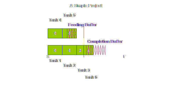
be better utilized, and we need less in total than we had before. The rule is
that we need only half as much aggregated buffer as we did as prior
non-aggregated safety. Therefore we
must halve the buffers (4). Let’s see what
this gives us.
Looking at it
another way, our new project duration is made up of 2/3rd’s task and 1/3rd
buffer. And this leads us to a more
generic buffer sizing rule. Regardless
of the task sizing rule that is used, the buffers
must be 50% of the task estimate.
The “completion buffer is 1/2 of the lead time of the (trimmed)
project” (7). Take care to
note; we now have a sequence, not a schedule.
Tasks 1, 2, 3, 4, and 6 are squashed up on the left; this doesn’t mean
each task is expected to be finished in the time allocated to each task, nor
that each will start immediately after the preceding one. Instead we still expect the normal range of
variation that we have experienced up until now, but that that variation will
be accommodated from the global buffers It’s taken us
a long time to get here but I hope that it was worth it. Before we
finish however, let’s work through a project using our new found
knowledge. Here is the project plan or
sequence. We have added a some numbers
to make it a little more clear how the plan progresses.
Let’s step it
out another step.
Do you see
what we mean about a sequence. This is
not a schedule, we don’t know at this moment when task 6 for instance will
begin, nor for that matter when it will be completed. Let’s step it
out once again.
Let’s see what
happens at the end.
Hopefully this
simple sketch shows you the nature of the buffer; it is there to be consumed
in some rough proportion to the tasks at hand. Its location ensures that we can average
out the over-runs and the under-runs.
By aggregating the safety we can be equally effective with less, and
thus the whole project can be completed, not only on time, but also in less
time than we might otherwise manage.
We are also dealing with a sequence rather than a schedule; the start
and finish dates are fixed, but everything else is free to move as needed to
accommodate the variation and uncertainty in the project as it unfolds. Buffering of
the project plan is just one aspect of Critical Chain Project
Management. We’ve labored it here,
because there are so many subtleties that need to be explained. It should be pointed out that strictly
speaking we currently have a buffered Critical Path, and in the next section
we will show the difference that converts it into a Critical Chain. Also we have spent a lot of time on an
aspect of project management which is essentially project planning. The greatest gains from Critical Chain
Project Management don’t come from the planning but rather from the
execution. Having a buffered Critical
Chain plan, and knowing how to monitor the buffer against the plan gives
project managers a degree of control that is unimaginable with Critical Path
Method – as we shall see in the next page. Most of the
problems in project operations, like production operations, must be
psychological – our competitors don’t seem to have undue inability to produce
similar products/services and yet we all seem to have similar problems along
the way. Treating the problem as
psychological and “of us” rather than “of them” helps us to more readily
frame the solution. To put it more
bluntly, if nothing else works at least we should be open to changing our own
thinking. Recognizing the implicit embedded
safety in each individual task and moving it to a more compact and globally
accessible buffer is an important step along this path. A project is
an “A” plant tipped on its side. Both
project operation buffers and production operation buffers in Theory of
Constraints are exactly the same animal.
The differences come from the fact that we ignore touch time in
production applications and include it in project applications. Project
buffers allow us to aggregate system safety in a few critical places where it
is available to all preceding tasks and thus allows the effective averaging
out of tasks that take longer durations than expected with those that take
shorter durations than expected.
Aggregated safety as global project buffers is in fact more than
adequate compared to the case where safety is distributed locally and
embedded within each task. Therefore
projects can be completed on-time and within 75% of the previous estimates. However, there is more than just buffers to
Critical Chain Project Management, and we must now turn our attention to
these. (1) Karl Buckridge, personal communication 2008. (2) Goldratt, E. M., (1998) Project Management the
TOC Way. Avraham Y. Goldratt Institute
Limited, pg 40. (3) Newbold, R.
C., (1998) Project management in the fast lane: applying the Theory of
Constraints. St. Lucie Press, pp
25-27. (4) Goldratt,
E. M., (1997) Critical chain. North
River Press, 246 pp. (5) Kendall, G. I., (2005) Viable Vision:
transforming total sales into net profits.
J. Ross Publishing, pg 79. (6) Leach, L.P.,
(2000) Critical chain project management.
Artech House Inc., pg 110. (7) Goldratt, E. M., (2003-2006) TOC insights into
project management and engineering.
Goldratt’s Marketing Group (software-based tutorial). This Webpage Copyright © 2008 - 2009 by Dr K. J.
Youngman |